|
Reference documentation for deal.II version 9.1.0-pre
|
|
Reference documentation for deal.II version 9.1.0-pre
|
This tutorial depends on step-5.
| Table of contents | |
|---|---|
This program is finally about one of the main features of deal.II: the use of adaptively (locally) refined meshes. The program is still based on step-4 and step-5, and, as you will see, it does not actually take very much code to enable adaptivity. Indeed, while we do a great deal of explaining, adaptive meshes can be added to an existing program with barely a dozen lines of additional code. The program shows what these lines are, as well as another important ingredient of adaptive mesh refinement (AMR): a criterion that can be used to determine whether it is necessary to refine a cell because the error is large on it, whether the cell can be coarsened because the error is particularly small on it, or whether we should just leave the cell as it is. We will discuss all of these issues in the following.
There are a number of ways how one can adaptively refine meshes. The basic structure of the overall algorithm is always the same and consists of a loop over the following steps:
For reasons that are probably lost to history (maybe that these functions used to be implemented in FORTRAN, a language that does not care about whether something is spelled in lower or UPPER case letters, with programmers often choosing upper case letters habitually), the loop above is often referenced in publications about mesh adaptivity as the SOLVE-ESTIMATE-MARK-REFINE loop (with this spelling).
Beyond this structure, however, there are a variety of ways to achieve this. Fundamentally, they differ in how exactly one generates one mesh from the previous one.
If one were to use triangles (which deal.II does not do), then there are two essential possibilities:
There are other variations of these approaches, but the important point is that they always generate a mesh where the lines where two cells touch are entire edges of both adjacent cells. With a bit of work, this strategy is readily adapted to three-dimensional meshes made from tetrahedra.
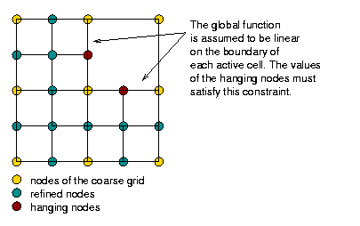
Neither of these methods works for quadrilaterals in 2d and hexahedra in 3d, or at least not easily. The reason is that the transition elements created out of the quadrilateral neighbors of a quadrilateral cell that is to be refined would be triangles, and we don't want this. Consequently, the approach to adaptivity chosen in deal.II is to use grids in which neighboring cells may differ in refinement level by one. This then results in nodes on the interfaces of cells which belong to one side, but are unbalanced on the other. The common term for these is “hanging nodes”, and these meshes then look like this in a very simple situation:
A more complicated two-dimensional mesh would look like this (and is discussed in the "Results" section below):

Finally, a three-dimensional mesh (from step-43) with such hanging nodes is shown here:

The first and third mesh are of course based on a square and a cube, but as the second mesh shows, this is not necessary. The important point is simply that we can refine a mesh independently of its neighbors (subject to the constraint that a cell can be only refined once more than its neighbors), but that we end up with these “hanging nodes” if we do this.
Now that you have seen what these adaptively refined meshes look like, you should ask why we would want to do this. After all, we know from theory that if we refine the mesh globally, the error will go down to zero as
\begin{align*} \|\nabla(u-u_h)\|_{\Omega} \le C h_\text{max}^p \| \nabla^{p+1} u \|_{\Omega}, \end{align*}
where \(C\) is some constant independent of \(h\) and \(u\), \(p\) is the polynomial degree of the finite element in use, and \(h_\text{max}\) is the diameter of the largest cell. So if the largest cell is important, then why would we want to make the mesh fine in some parts of the domain but not all?
The answer lies in the observation that the formula above is not optimal. In fact, some more work shows that the following is a better estimate (which you should compare to the square of the estimate above):
\begin{align*} \|\nabla(u-u_h)\|_{\Omega}^2 \le C \sum_K h_K^{2p} \| \nabla^{p+1} u \|^2_K. \end{align*}
(Because \(h_K\le h_\text{max}\), this formula immediately implies the previous one if you just pull the mesh size out of the sum.) What this formula suggests is that it is not necessary to make the largest cell small, but that the cells really only need to be small where \(\| \nabla^{p+1} u \|_K\) is large! In other words: The mesh really only has to be fine where the solution has large variations, as indicated by the \(p+1\)st derivative. This makes intuitive sense: if, for example, we use a linear element \(p=1\), then places where the solution is nearly linear (as indicated by \(\nabla^2 u\) being small) will be well resolved even if the mesh is coarse. Only those places where the second derivative is large will be poorly resolved by large elements, and consequently that's where we should make the mesh small.
Of course, this a priori estimate is not very useful in practice since we don't know the exact solution \(u\) of the problem, and consequently, we cannot compute \(\nabla^{p+1}u\). But, and that is the approach commonly taken, we can compute numerical approximations of \(\nabla^{p+1}u\) based only on the discrete solution \(u_h\) that we have computed before. We will discuss this in slightly more detail below. This will then help us determine which cells have a large \(p+1\)st derivative, and these are then candidates for refining the mesh.
The methods using triangular meshes mentioned above go to great lengths to make sure that each vertex is a vertex of all adjacent cells – i.e., that there are no hanging nodes. This then automatically makes sure that we can define shape functions in such a way that they are globally continuous (if we use the common \(Q_p\) Lagrange finite element methods we have been using so far in the tutorial programs, as represented by the FE_Q class).
On the other hand, if we define shape functions on meshes with hanging nodes, we may end up with shape functions that are not continuous. To see this, think about the situation above where the top right cell is not refined, and consider for a moment the use of a bilinear finite element. In that case, the shape functions associated with the hanging nodes are defined in the obvious way on the two small cells adjacent to each of the hanging nodes. But how do we extend them to the big adjacent cells? Clearly, the function's extension to the big cell cannot be bilinear because then it needs to be linear along each edge of the large cell, and that means that it needs to be zero on the entire edge because it needs to be zero on the two vertices of the large cell on that edge. But it is not zero at the hanging node itself when seen from the small cells' side – so it is not continuous. The following three figures show three of the shape functions along the edges in question that turn out to not be continuous when defined in the usual way simply based on the cells they are adjacent to:
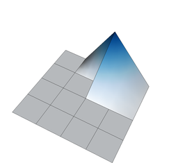
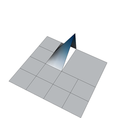
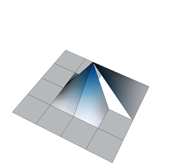
But we do want the finite element solution to be continuous so that we have a “conforming finite element method” where the discrete finite element space is a proper subset of the \(H^1\) function space in which we seek the solution of the Laplace equation. To guarantee that the global solution is continuous at these nodes as well, we have to state some additional constraints on the values of the solution at these nodes. The trick is to realize that while the shape functions shown above are discontinuous (and consequently an arbitrary linear combination of them is also discontinuous), that linear combinations in which the shape functions are added up as \(u_h(\mathbf x)=\sum_j U_j \varphi_j(\mathbf x)\) can be continuous if the coefficients \(U_j\) satisfy certain relationships. In other words, the coefficients \(U_j\) can not be chosen arbitrarily but have to satisfy certain constraints so that the function \(u_h\) is in fact continuous. What these constraints have to look is relatively easy to understand conceptually, but the implementation in software is complicated and takes several thousand lines of code. On the other hand, in user code, it is only about half a dozen lines you have to add when dealing with hanging nodes.
In the program below, we will show how we can get these constraints from deal.II, and how to use them in the solution of the linear system of equations. Before going over the details of the program below, you may want to take a look at the Constraints on degrees of freedom documentation module that explains how these constraints can be computed and what classes in deal.II work on them.
The practice of hanging node constraints is rather simpler than the theory we have outlined above. In reality, you will really only have to add about half a dozen lines of additional code to a program like step-4 to make it work with adaptive meshes that have hanging nodes. The interesting part about this is that it is entirely independent of the equation you are solving: The algebraic nature of these constraints has nothing to do with the equation and only depends on the choice of finite element. As a consequence, the code to deal with these constraints is entirely contained in the deal.II library itself, and you do not need to worry about the details.
The steps you need to make this work are essentially like this:
These four steps are really all that is necessary – it's that simple from a user perspective. The fact that, in the function calls mentioned above, you will run through several thousand lines of not-so-trivial code is entirely immaterial to this: In user code, there are really only four additional steps.
The next question, now that we know how to deal with meshes that have these hanging nodes is how we obtain them.
A simple way has already been shown in step-1: If you know where it is necessary to refine the mesh, then you can create one by hand. But in reality, we don't know this: We don't know the solution of the PDE up front (because, if we did, we wouldn't have to use the finite element method), and consequently we do not know where it is necessary to add local mesh refinement to better resolve areas where the solution has strong variations. But the discussion above shows that maybe we can get away with using the discrete solution \(u_h\) on one mesh to estimate the derivatives \(\nabla^{p+1} u\), and then use this to determine which cells are too large and which already small enough. We can then generate a new mesh from the current one using local mesh refinement. If necessary, this step is then repeated until we are happy with our numerical solution – or, more commonly, until we run out of computational resources or patience.
So that's exactly what we will do. The locally refined grids are produced using an error estimator which estimates the energy error for numerical solutions of the Laplace operator. Since it was developed by Kelly and co-workers, we often refer to it as the “Kelly refinement indicator” in the library, documentation, and mailing list. The class that implements it is called KellyErrorEstimator, and there is a great deal of information to be found in the documentation of that class that need not be repeated here. The summary, however, is that the class computes a vector with as many entries as there are active cells, and where each entry contains an estimate of the error on that cell. This estimate is then used to refine the cells of the mesh: those cells that have a large error will be marked for refinement, those that have a particularly small estimate will be marked for coarsening. We don't have to do this by hand: The functions in namespace GridRefinement will do all of this for us once we have obtained the vector of error estimates.
It is worth noting that while the Kelly error estimator was developed for Laplace's equation, it has proven to be a suitable tool to generate locally refined meshes for a wide range of equations, not even restricted to elliptic only problems. Although it will create non-optimal meshes for other equations, it is often a good way to quickly produce meshes that are well adapted to the features of solutions, such as regions of great variation or discontinuities.
It turns out that one can see Dirichlet boundary conditions as just another constraint on the degrees of freedom. It's a particularly simple one, indeed: If \(j\) is a degree of freedom on the boundary, with position \(\mathbf x_j\), then imposing the boundary condition \(u=g\) on \(\partial\Omega\) simply yields the constraint \(U_j=g({\mathbf x}_j)\).
The AffineConstraints can handle such constraints as well, which makes it convenient to let the same object we use for hanging node constraints also deal with these Dirichlet boundary conditions. This way, we don't need to apply the boundary conditions after assembly (like we did in the earlier steps). All that is necessary is that we call the variant of VectorTools::interpolate_boundary_values() that returns its information in a AffineConstraints object, rather than the std::map we have used in previous tutorial programs.
Since the concepts used for locally refined grids are so important, we do not show much other material in this example. The most important exception is that we show how to use biquadratic elements instead of the bilinear ones which we have used in all previous examples. In fact, the use of higher order elements is accomplished by only replacing three lines of the program, namely the initialization of the fe member variable in the constructor of the main class of this program, and the use of an appropriate quadrature formula in two places. The rest of the program is unchanged.
The only other new thing is a method to catch exceptions in the main function in order to output some information in case the program crashes for some reason. This is discussed below in more detail.
The first few files have already been covered in previous examples and will thus not be further commented on.
From the following include file we will import the declaration of H1-conforming finite element shape functions. This family of finite elements is called FE_Q, and was used in all examples before already to define the usual bi- or tri-linear elements, but we will now use it for bi-quadratic elements:
We will not read the grid from a file as in the previous example, but generate it using a function of the library. However, we will want to write out the locally refined grids (just the grid, not the solution) in each step, so we need the following include file instead of grid_in.h:
When using locally refined grids, we will get so-called hanging nodes. However, the standard finite element methods assumes that the discrete solution spaces be continuous, so we need to make sure that the degrees of freedom on hanging nodes conform to some constraints such that the global solution is continuous. We are also going to store the boundary conditions in this object. The following file contains a class which is used to handle these constraints:
In order to refine our grids locally, we need a function from the library that decides which cells to flag for refinement or coarsening based on the error indicators we have computed. This function is defined here:
Finally, we need a simple way to actually compute the refinement indicators based on some error estimate. While in general, adaptivity is very problem-specific, the error indicator in the following file often yields quite nicely adapted grids for a wide class of problems.
Finally, this is as in previous programs:
Step6 class templateThe main class is again almost unchanged. Two additions, however, are made: we have added the refine_grid function, which is used to adaptively refine the grid (instead of the global refinement in the previous examples), and a variable which will hold the constraints. In addition, we have added a destructor to the class for reasons that will become clear when we discuss its implementation.
This is the new variable in the main class. We need an object which holds a list of constraints to hold the hanging nodes and the boundary conditions.
The sparsity pattern and sparse matrix are deliberately declared in the opposite of the order used in step-2 through step-5 to demonstrate the primary use of the Subscriptor and SmartPointer classes.
The implementation of nonconstant coefficients is copied verbatim from step-5:
Step6 class implementationThe constructor of this class is mostly the same as before, but this time we want to use the quadratic element. To do so, we only have to replace the constructor argument (which was 1 in all previous examples) by the desired polynomial degree (here 2):
Here comes the added destructor of the class. Some objects in deal.II store pointers to other objects: in particular a SparseMatrix stores a SmartPointer pointing to the SparsityPattern with which it was initialized. This example deliberately declares the SparseMatrix before the SparsityPattern to make this dependency clearer. Of course we could have left this order unchanged, but we would like to show what happens if the order is reversed since this produces a rather nasty side-effect and results in an error which is difficult to track down if one does not know what happens.
What happens is the following: when we initialize a SparseMatrix, the matrix stores a pointer to the provided SparsityPattern instead of copying it. Since this pointer is used until either another SparsityPattern is attached or the SparseMatrix is destructed, it would be unwise to allow the SparsityPattern to be destructed before the SparseMatrix. To disallow this, the SparseMatrix increases a counter inside the SparsityPattern which counts how many objects use it (this is what the Subscriptor/SmartPointer class pair is used for, in case you want something like this for your own programs; see step-7 for a more complete discussion of this topic). If we try to destroy the object while the counter is larger than zero then the program will either abort (the default) or print an error message and continue: see the documentation of AssertNothrow for more details. In either case the program contains a bug and this facility will, hopefully, point out where.
To be fair, such errors due to object dependencies are not particularly popular among programmers using deal.II, since they only tell us that something is wrong, namely that some other object is still using the object that is presently being destroyed, but most of the time not which object is still using it. It is therefore often rather time-consuming to find out where the problem exactly is, although it is then usually straightforward to remedy the situation. However, we believe that the effort to find invalid pointers to objects that no longer exist is less if the problem is detected once the pointer becomes invalid, rather than when non-existent objects are actually accessed again, since then usually only invalid data is accessed, but no error is immediately raised.
Coming back to the present situation, if we did not write this destructor, then the compiler would generate code that triggers exactly the behavior described above. The reason is that member variables of the Step6 class are destroyed bottom-up (i.e., in reverse order of their declaration in the class), as always in C++. Thus, the SparsityPattern will be destroyed before the SparseMatrix, since its declaration is below the declaration of the sparsity pattern. This triggers the situation above, and without manual intervention the program will abort when the SparsityPattern is destroyed. What needs to be done is to tell the SparseMatrix to release its pointer to the SparsityPattern. Of course, the SparseMatrix will only release its pointer if it really does not need the SparsityPattern any more. For this purpose, the SparseMatrix class has a function SparseMatrix::clear() which resets the object to its default-constructed state by deleting all data and resetting its pointer to the SparsityPattern to 0. After this, you can safely destruct the SparsityPattern since its internal counter will be zero.
We show the output of the other case (where we do not call SparseMatrix::clear()) in the results section below.
The next function sets up all the variables that describe the linear finite element problem, such as the DoFHandler, matrices, and vectors. The difference to what we did in step-5 is only that we now also have to take care of hanging node constraints. These constraints are handled almost exclusively by the library, i.e. you only need to know that they exist and how to get them, but you do not have to know how they are formed or what exactly is done with them.
At the beginning of the function, you find all the things that are the same as in step-5: setting up the degrees of freedom (this time we have quadratic elements, but there is no difference from a user code perspective to the linear – or any other degree, for that matter – case), generating the sparsity pattern, and initializing the solution and right hand side vectors. Note that the sparsity pattern will have significantly more entries per row now, since there are now 9 degrees of freedom per cell (rather than only four), that can couple with each other.
We may now populate the AffineConstraints object with the hanging node constraints. Since we will call this function in a loop we first clear the current set of constraints from the last system and then compute new ones:
Now we are ready to interpolate the boundary values with indicator 0 (the whole boundary) and store the resulting constraints in our constraints object. Note that we do not to apply the boundary conditions after assembly, like we did in earlier steps: instead we put all constraints on our function space in the AffineConstraints. We can add constraints to the AffineConstraints in either order: if two constraints conflict then the constraint matrix either abort or throw an exception via the Assert macro.
After all constraints have been added, they need to be sorted and rearranged to perform some actions more efficiently. This postprocessing is done using the close() function, after which no further constraints may be added any more:
Now we first build our compressed sparsity pattern like we did in the previous examples. Nevertheless, we do not copy it to the final sparsity pattern immediately. Note that we call a variant of make_sparsity_pattern that takes the AffineConstraints object as the third argument. We are letting the routine know that we will never write into the locations given by constraints by setting the argument keep_constrained_dofs to false (in other words, that we will never write into entries of the matrix that correspond to constrained degrees of freedom). If we were to condense the constraints after assembling, we would have to pass true instead because then we would first write into these locations only to later set them to zero again during condensation.
Now all non-zero entries of the matrix are known (i.e. those from regularly assembling the matrix and those that were introduced by eliminating constraints). We may copy our intermediate object to the sparsity pattern:
We may now, finally, initialize the sparse matrix:
Next, we have to assemble the matrix again. There are two code changes compared to step-5:
First, we have to use a higher-order quadrature formula to account for the higher polynomial degree in the finite element shape functions. This is easy to change: the constructor of the QGauss class takes the number of quadrature points in each space direction. Previously, we had two points for bilinear elements. Now we should use three points for biquadratic elements.
Second, to copy the local matrix and vector on each cell into the global system, we are no longer using a hand-written loop. Instead, we use AffineConstraints::distribute_local_to_global() that internally executes this loop while performing Gaussian elimination on rows and columns corresponding to constrained degrees on freedom.
The rest of the code that forms the local contributions remains unchanged. It is worth noting, however, that under the hood several things are different than before. First, the variables dofs_per_cell and n_q_points now are 9 each, where they were 4 before. Introducing such variables as abbreviations is a good strategy to make code work with different elements without having to change too much code. Secondly, the fe_values object of course needs to do other things as well, since the shape functions are now quadratic, rather than linear, in each coordinate variable. Again, however, this is something that is completely handled by the library.
Finally, transfer the contributions from cell_matrix and cell_rhs into the global objects.
Now we are done assembling the linear system. The constraint matrix took care of applying the boundary conditions and also eliminated hanging node constraints. The constrained nodes are still in the linear system (there is a nonzero entry, chosen in a way that the matrix is well conditioned, on the diagonal of the matrix and all other entries for this line are set to zero) but the computed values are invalid (i.e., the correspond entry in system_rhs is currently meaningless). We compute the correct values for these nodes at the end of the solve function.
We continue with gradual improvements. The function that solves the linear system again uses the SSOR preconditioner, and is again unchanged except that we have to incorporate hanging node constraints. As mentioned above, the degrees of freedom from the AffineConstraints object corresponding to hanging node constraints and boundary values have been removed from the linear system by giving the rows and columns of the matrix a special treatment. This way, the values for these degrees of freedom have wrong, but well-defined values after solving the linear system. What we then have to do is to use the constraints to assign to them the values that they should have. This process, called distributing constraints, computes the values of constrained nodes from the values of the unconstrained ones, and requires only a single additional function call that you find at the end of this function:
We use a sophisticated error estimation scheme to refine the mesh instead of global refinement. We will use the KellyErrorEstimator class which implements an error estimator for the Laplace equation; it can in principle handle variable coefficients, but we will not use these advanced features, but rather use its most simple form since we are not interested in quantitative results but only in a quick way to generate locally refined grids.
Although the error estimator derived by Kelly et al. was originally developed for the Laplace equation, we have found that it is also well suited to quickly generate locally refined grids for a wide class of problems. This error estimator uses the solution gradient's jump at cell faces (which is a measure for the second derivatives) and scales it by the size of the cell. It is therefore a measure for the local smoothness of the solution at the place of each cell and it is thus understandable that it yields reasonable grids also for hyperbolic transport problems or the wave equation as well, although these grids are certainly suboptimal compared to approaches specially tailored to the problem. This error estimator may therefore be understood as a quick way to test an adaptive program.
The way the estimator works is to take a DoFHandler object describing the degrees of freedom and a vector of values for each degree of freedom as input and compute a single indicator value for each active cell of the triangulation (i.e. one value for each of the active cells). To do so, it needs two additional pieces of information: a face quadrature formula, i.e., a quadrature formula on dim-1 dimensional objects. We use a 3-point Gauss rule again, a choice that is consistent and appropriate with the bi-quadratic finite element shape functions in this program. (What constitutes a suitable quadrature rule here of course depends on knowledge of the way the error estimator evaluates the solution field. As said above, the jump of the gradient is integrated over each face, which would be a quadratic function on each face for the quadratic elements in use in this example. In fact, however, it is the square of the jump of the gradient, as explained in the documentation of that class, and that is a quartic function, for which a 3 point Gauss formula is sufficient since it integrates polynomials up to order 5 exactly.)
Secondly, the function wants a list of boundary indicators for those boundaries where we have imposed Neumann values of the kind \(\partial_n u(\mathbf x) = h(\mathbf x)\), along with a function \(h(\mathbf x)\) for each such boundary. This information is represented by a map from boundary indicators to function objects describing the Neumann boundary values. In the present example program, we do not use Neumann boundary values, so this map is empty, and in fact constructed using the default constructor of the map in the place where the function call expects the respective function argument.
The output is a vector of values for all active cells. While it may make sense to compute the value of a solution degree of freedom very accurately, it is usually not necessary to compute the error indicator corresponding to the solution on a cell particularly accurately. We therefore typically use a vector of floats instead of a vector of doubles to represent error indicators.
The above function returned one error indicator value for each cell in the estimated_error_per_cell array. Refinement is now done as follows: refine those 30 per cent of the cells with the highest error values, and coarsen the 3 per cent of cells with the lowest values.
One can easily verify that if the second number were zero, this would approximately result in a doubling of cells in each step in two space dimensions, since for each of the 30 per cent of cells, four new would be replaced, while the remaining 70 per cent of cells remain untouched. In practice, some more cells are usually produced since it is disallowed that a cell is refined twice while the neighbor cell is not refined; in that case, the neighbor cell would be refined as well.
In many applications, the number of cells to be coarsened would be set to something larger than only three per cent. A non-zero value is useful especially if for some reason the initial (coarse) grid is already rather refined. In that case, it might be necessary to refine it in some regions, while coarsening in some other regions is useful. In our case here, the initial grid is very coarse, so coarsening is only necessary in a few regions where over-refinement may have taken place. Thus a small, non-zero value is appropriate here.
The following function now takes these refinement indicators and flags some cells of the triangulation for refinement or coarsening using the method described above. It is from a class that implements several different algorithms to refine a triangulation based on cell-wise error indicators.
After the previous function has exited, some cells are flagged for refinement, and some other for coarsening. The refinement or coarsening itself is not performed by now, however, since there are cases where further modifications of these flags is useful. Here, we don't want to do any such thing, so we can tell the triangulation to perform the actions for which the cells are flagged:
At the end of computations on each grid, and just before we continue the next cycle with mesh refinement, we want to output the results from this cycle.
We have already seen in step-1 how this can be achieved for the mesh itself. The only thing we have to change is the generation of the file name, since it should contain the number of the present refinement cycle provided to this function as an argument. To this end, we simply append the number of the refinement cycle as a string to the file name.
We also output the solution in the same way as we did before, with a similarly constructed file name.
The final function before main() is again the main driver of the class, run(). It is similar to the one of step-5, except that we generate a file in the program again instead of reading it from disk, in that we adaptively instead of globally refine the mesh, and that we output the solution on the final mesh in the present function.
The first block in the main loop of the function deals with mesh generation. If this is the first cycle of the program, instead of reading the grid from a file on disk as in the previous example, we now again create it using a library function. The domain is again a circle, which is why we have to provide a suitable boundary object as well. We place the center of the circle at the origin and have the radius be one (these are the two hidden arguments to the function, which have default values).
You will notice by looking at the coarse grid that it is of inferior quality than the one which we read from the file in the previous example: the cells are less equally formed. However, using the library function this program works in any space dimension, which was not the case before.
In case we find that this is not the first cycle, we want to refine the grid. Unlike the global refinement employed in the last example program, we now use the adaptive procedure described above.
The rest of the loop looks as before:
main functionThe main function is unaltered in its functionality from the previous example, but we have taken a step of additional caution. Sometimes, something goes wrong (such as insufficient disk space upon writing an output file, not enough memory when trying to allocate a vector or a matrix, or if we can't read from or write to a file for whatever reason), and in these cases the library will throw exceptions. Since these are run-time problems, not programming errors that can be fixed once and for all, this kind of exceptions is not switched off in optimized mode, in contrast to the Assert macro which we have used to test against programming errors. If uncaught, these exceptions propagate the call tree up to the main function, and if they are not caught there either, the program is aborted. In many cases, like if there is not enough memory or disk space, we can't do anything but we can at least print some text trying to explain the reason why the program failed. A way to do so is shown in the following. It is certainly useful to write any larger program in this way, and you can do so by more or less copying this function except for the try block that actually encodes the functionality particular to the present application.
The general idea behind the layout of this function is as follows: let's try to run the program as we did before...
...and if this should fail, try to gather as much information as possible. Specifically, if the exception that was thrown is an object of a class that is derived from the C++ standard class exception, then we can use the what member function to get a string which describes the reason why the exception was thrown.
The deal.II exception classes are all derived from the standard class, and in particular, the exc.what() function will return approximately the same string as would be generated if the exception was thrown using the Assert macro. You have seen the output of such an exception in the previous example, and you then know that it contains the file and line number of where the exception occurred, and some other information. This is also what the following statements would print.
Apart from this, there isn't much that we can do except exiting the program with an error code (this is what the return 1; does):
If the exception that was thrown somewhere was not an object of a class derived from the standard exception class, then we can't do anything at all. We then simply print an error message and exit.
If we got to this point, there was no exception which propagated up to the main function (there may have been exceptions, but they were caught somewhere in the program or the library). Therefore, the program performed as was expected and we can return without error.
The output of the program looks as follows:
As intended, the number of cells roughly doubles in each cycle. The number of degrees is slightly more than four times the number of cells; one would expect a factor of exactly four in two spatial dimensions on an infinite grid (since the spacing between the degrees of freedom is half the cell width: one additional degree of freedom on each edge and one in the middle of each cell), but it is larger than that factor due to the finite size of the mesh and due to additional degrees of freedom which are introduced by hanging nodes and local refinement.
The final solution, as written by the program at the end of the run() function, looks as follows:

In each cycle, the program furthermore writes the grid in EPS format. These are shown in the following:


It is clearly visible that the region where the solution has a kink, i.e. the circle at radial distance 0.5 from the center, is refined most. Furthermore, the central region where the solution is very smooth and almost flat, is almost not refined at all, but this results from the fact that we did not take into account that the coefficient is large there. The region outside is refined rather arbitrarily, since the second derivative is constant there and refinement is therefore mostly based on the size of the cells and their deviation from the optimal square.
For completeness, we show what happens if the code we commented about in the destructor of the Step6 class is omitted from this example:
From the above error message, we conclude that something is still using an object with type N6dealii15SparsityPatternE. This is of course the "mangled" name for SparsityPattern. The mangling works as follows: the N6 indicates a namespace with six characters (i.e., dealii) and the 15 indicates the number of characters of the template class (i.e., SparsityPattern).
From this we can already glean a little bit who is the culprit here, and who the victim: The one object that still uses the SparsityPattern is the SparseMatrix.
The stacktrace gives an indication of where the problem happened. We see that the AssertNothrow macro was triggered in the destructor of the SparseMatrix class (which inherits from Subscriptor) that was called through a few more functions from the destructor of the Step6 class, exactly where we have commented out the call to SparseMatrix::clear().
One thing that is always worth playing around with if one solves problems of appreciable size (much bigger than the one we have here) is to try different solvers or preconditioners. In the current case, the linear system is symmetric and positive definite, which makes the CG algorithm pretty much the canonical choice for solving. However, the SSOR preconditioner we use in the solve() function is up for grabs.
In deal.II, it is relatively simple to change the preconditioner. For example, by changing the existing lines of code
into
we can try out different relaxation parameters for SSOR. By using (you have to also add the header file lac/sparse_ilu.h to the include list at the top of the file)
we can use Jacobi as a preconditioner. And by using
we can use a simple incomplete LU decomposition without any thresholding or strengthening of the diagonal.
Using these various different preconditioners, we can compare the number of CG iterations needed (available through the solver_control.last_step() call, see step-4) as well as CPU time needed (using the Timer class, discussed, for example, in step-12) and get the following results (left: iterations; right: CPU time):

| 
|
As we can see, all preconditioners behave pretty much the same on this simple problem, with the number of iterations growing like \({\cal O}(N^{1/2})\) and because each iteration requires around \({\cal O}(N)\) operations the total CPU time grows like \({\cal O}(N^{3/2})\) (for the few smallest meshes, the CPU time is so small that it doesn't record). Note that even though it is the simplest method, Jacobi is the fastest for this problem.
The situation changes slightly when the finite element is not a bi-quadratic one as set in the constructor of this program, but a bi-linear one. If one makes this change, the results are as follows:

| 
|
In other words, while the increase in iterations and CPU time is as before, Jacobi is now the method that requires the most iterations; it is still the fastest one, however, owing to the simplicity of the operations it has to perform. This is not to say that Jacobi is actually a good preconditioner – for problems of appreciable size, it is definitely not, and other methods will be substantially better – but really only that it is fast because its implementation is so simple that it can compensate for a larger number of iterations.
The message to take away from this is not that simplicity in preconditioners is always best. While this may be true for the current problem, it definitely is not once we move to more complicated problems (elasticity or Stokes, for examples step-8 or step-22). Secondly, all of these preconditioners still lead to an increase in the number of iterations as the number \(N\) of degrees of freedom grows, for example \({\cal O}(N^\alpha)\); this, in turn, leads to a total growth in effort as \({\cal O}(N^{1+\alpha})\) since each iteration takes \({\cal O}(N)\) work. This behavior is undesirable: we would really like to solve linear systems with \(N\) unknowns in a total of \({\cal O}(N)\) work; there is a class of preconditioners that can achieve this, namely geometric (step-16, step-37, step-39) or algebraic multigrid (step-31, step-40, and several others) preconditioners. They are, however, significantly more complex than the preconditioners outlined above.
Finally, the last message to take home is that when the data shown above was generated (in 2018), linear systems with 100,000 unknowns are easily solved on a desktop machine in about a second, making the solution of relatively simple 2d problems even to very high accuracy not that big a task as it used to be even in the past. At the time, the situation for 3d problems was entirely different, but even that has changed substantially in the intervening time – though solving problems in 3d to high accuracy remains a challenge.
If you look at the meshes above, you will see even though the domain is the unit disk, and the jump in the coefficient lies along a circle, the cells that make up the mesh do not track this geometry well. The reason, already hinted at in step-1, is that by default the Triangulation class only sees a bunch of coarse grid cells but has, of course, no real idea what kind of geometry they might represent when looked at together. For this reason, we need to tell the Triangulation what to do when a cell is refined: where should the new vertices at the edge midpoints and the cell midpoint be located so that the child cells better represent the desired geometry than the parent cell.
In the code above, we already do this for faces that sit at the boundary: this happens automatically since we use GridGenerator::hyper_ball, which attaches a SphericalManifold to the boundary of the domain. To make the mesh interior also track a circular domain, we need to work a bit harder, though. First, recall that our coarse mesh consists of a central square cell and four cells around it. Now first consider what would happen if we also attached the SphericalManifold object not only to the four exterior faces but also the four cells at the perimeter as well as all of their faces. We can do this by adding the following snippet (testing that the center of a cell is larger than a small multiple, say one tenth, of the cell diameter away from center of the mesh only fails for the central square of the mesh):
After a few global refinement steps, this would lead to a mesh of the following kind:

This is not a good mesh: the central cell has been refined in such a way that the children located in the four corners of the original central cell degenerate: they all tend towards triangles as mesh refinement continues. This means that the Jacobian matrix of the transformation from reference cell to actual cell degenerates for these cells, and because all error estimates for finite element solutions contain the norm of the inverse of the Jacobian matrix, you will get very large errors on these cells and, in the limit as mesh refinement, a loss of convergence order because the cells in these corners become worse and worse under mesh refinement.
So we need something smarter. To this end, consider the following solution originally developed by Konstantin Ladutenko. We will use the following code:
This code then generates the following, much better sequence of meshes:


Creating good meshes, and in particular making them fit the geometry you want, is a complex topic in itself. You can find much more on this in step-49, step-53, and step-54, among other tutorial programs that cover the issue. Information on curved domains can also be found in the documentation module on Manifold descriptions.
Why does it make sense to choose a mesh that tracks the internal interface? There are a number of reasons, but the most essential one comes down to what we actually integrate in our bilinear form. Conceptually, we want to integrate the term \(A_{ij}^K=\int_K a(\mathbf x) \nabla \varphi_i(\mathbf x) \nabla \varphi_j(\mathbf x) ; dx\) as the contribution of cell \(K\) to the matrix entry \(A_{ij}\). We can not compute it exactly and have to resort to quadrature. We know that quadrature is accurate if the integrand is smooth. That is because quadrature in essence computes a polynomial approximation to the integrand that coincides with the integrand in the quadrature points, and then computes the volume under this polynomial as an approximation to the volume under the original integrand. This polynomial interpolant is accurate if the integrand is smooth on a cell, but it is usually rather inaccurate if the integrand is discontinuous on a cell.
Consequently, it is worthwhile to align cells in such a way that the interfaces across which the coefficient is discontinuous are aligned with cell interfaces. This way, the coefficient is constant on each cell, following which the integrand will be smooth, and its polynomial approximation and the quadrature approximation of the integral will both be accurate. Note that such an alignment is common in many practical cases, so deal.II provides a number of functions (such as material_id) to help manage such a scenario. Refer to step-28 and step-46 for examples of how material id's can be applied.
Finally, let us consider the case of a coefficient that has a smooth and non-uniform distribution in space. We can repeat once again all of the above discussion on the representation of such a function with the quadrature. So, to simulate it accurately there are a few readily available options: you could reduce the cell size, increase the order of the polynomial used in the quadrature formula, select a more appropriate quadrature formula, or perform a combination of these steps. The key is that providing the best fit of the coefficient's spatial dependence with the quadrature polynomial will lead to a more accurate finite element solution of the PDE.
From a mathematical perspective, solutions of the Laplace equation
\[ -\Delta u = f \]
on smoothly bounded, convex domains are known to be smooth themselves. The exact degree of smoothness, i.e., the function space in which the solution lives, depends on how smooth exactly the boundary of the domain is, and how smooth the right hand side is. Some regularity of the solution may be lost at the boundary, but one generally has that the solution is twice more differentiable in compact subsets of the domain than the right hand side. If, in particular, the right hand side satisfies \(f\in C^\infty(\Omega)\), then \(u \in C^\infty(\Omega_i)\) where \(\Omega_i\) is any compact subset of \(\Omega\) ( \(\Omega\) is an open domain, so a compact subset needs to keep a positive distance from \(\partial\Omega\)).
The situation we chose for the current example is different, however: we look at an equation with a non-constant coefficient \(a(\mathbf x)\):
\[ -\nabla \cdot (a \nabla u) = f. \]
Here, if \(a\) is not smooth, then the solution will not be smooth either, regardless of \(f\). In particular, we expect that wherever \(a\) is discontinuous along a line (or along a plane in 3d), the solution will have a kink. This is easy to see: if for example \(f\) is continuous, then \(f=-\nabla \cdot (a \nabla u)\) needs to be continuous. This means that \(a \nabla u\) must be continuously differentiable (not have a kink). Consequently, if \(a\) has a discontinuity, then \(\nabla u\) must have an opposite discontinuity so that the two exactly cancel and their product yields a function without a discontinuity. But for \(\nabla u\) to have a discontinuity, \(u\) must have a kink. This is of course exactly what is happening in the current example, and easy to observe in the pictures of the solution.
In general, if the coefficient \(a(\mathbf x)\) is discontinuous along a line in 2d, or a plane in 3d, then the solution may have a kink, but the gradient of the solution will not go to infinity. That means, that the solution is at least still in the space \(W^{1,\infty}\). On the other hand, we know that in the most extreme cases – i.e., where the domain has reentrant corners, the right hand side only satisfies \(f\in H^{-1}\), or the coefficient \(a\) is only in \(L^\infty\) – all we can expect is that \(u\in H^1\), a much larger space than \(W^{1,\infty}\). It is not very difficult to create cases where the solution is in a space \(H^{1+s}\) where we can get \(s\) to become as small as we want. Such cases are often used to test adaptive finite element methods because the mesh will have to resolve the singularity that causes the solution to not be in \(W^{1,\infty}\) any more.
The typical example one uses for this is called the Kellogg problem (referring to the paper "On the Poisson equation with intersecting interfaces" by R. B. Kellogg, Applicable Analysis, vol. 4, pp. 101-129, 1974), which in the commonly used form has a coefficient \(a(\mathbf x)\) that has different values in the four quadrants of the plane (or eight different values in the octants of \({\mathbb R}^3\)). The exact degree of regularity (the \(s\) in the index of the Sobolev space above) depends on the values of \(a(\mathbf x)\) coming together at the origin, and by choosing the jumps large enough, the regularity of the solution can be made as close as desired to \(H^1\).
To implement something like this, one could replace the coefficient function by the following (shown here only for the 2d case):
(Adding the Assert at the end ensures that either an exception is thrown or that the program aborts if we ever get to that point – which of course we shouldn't, but this is a good way to insure yourself: we all make mistakes by sometimes not thinking of all cases, for example by checking for p[0] to be less than and greater than zero, rather than greater-or-equal to zero, and thereby forgetting some cases that would otherwise lead to bugs that are awkward to find. The return 0; at the end is only there to avoid compiler warnings that the function does not end in a return statement – the compiler cannot see that the function would never actually get to that point because of the preceding Assert statement.)
By playing with such cases where four or more sectors come together and on which the coefficient has different values, one can construct cases where the solution has singularities at the origin. One can also see how the meshes are refined in such cases.
 1.8.11

