|
Reference documentation for deal.II version 9.1.0-pre
|
|
Reference documentation for deal.II version 9.1.0-pre
|
This tutorial depends on step-49.
| Table of contents | |
|---|---|
This program was contributed by Wolfgang Bangerth and Luca Heltai, using data provided by D. Sarah Stamps.
Partial differential equations for realistic problems are often posed on domains with complicated geometries. To provide just a few examples, consider these cases:
This program is therefore devoted to showing how one deals with complex geometries using a concrete application. In particular, what it shows is how we make a mesh fit the domain we want to solve on. On the other hand, what the program does not show is how to create a coarse for a domain. The process to arrive at a coarse mesh is called "mesh generation" and there are a number of high-quality programs that do this much better than we could ever implement. However, deal.II does have the ability to read in meshes in many formats generated by mesh generators and then make them fit a given shape, either by deforming a mesh or refining it a number of times until it fits. The deal.II Frequently Asked Questions page referenced from http://www.dealii.org/ provides resources to mesh generators.
Let us assume that you have a complex domain and that you already have a coarse mesh that somehow represents the general features of the domain. Then there are two situations in which it is necessary to describe to a deal.II program the details of your geometry:
In both cases, we need a way to provide information about the geometry of the domain at the level of an individual cell, its faces and edges. This is where the Manifold class comes into play. Manifold is an abstract base class that only defines an interface by which the Triangulation and Mapping classes can query geometric information about the domain. Conceptually, Manifold sees the world in a way not dissimilar to how the mathematical subdiscipline geometry sees it: a domain is essentially just a collection of points that is somehow equipped with the notion of a distance between points so that we can obtain a point "in the middle" of some other points.
deal.II provides a number of classes that implement the interface provided by Manifold for a variety of common geometries. On the other hand, in this program we will consider only a very common and much simpler case, namely the situation where (a part of) the domain we want to solve on can be described by transforming a much simpler domain (we will call this the "reference domain"). In the language of mathematics, this means that the (part of the) domain is a chart. Charts are described by a smooth function that maps from the simpler domain to the chart (the "push-forward" function) and its inverse (the "pull-back" function). If the domain as a whole is not a chart (e.g., the surface of a sphere), then it can often be described as a collection of charts (e.g., the northern hemisphere and the southern hemisphere are each charts) and the domain can then be describe by an atlas.
If a domain can be decomposed into an atlas, all we need to do is provide the pull-back and push-forward functions for each of the charts. In deal.II, this means providing a class derived from ChartManifold, and this is precisely what we will do in this program.
To illustrate how one describes geometries using charts in deal.II, we will consider a case that originates in an application of the ASPECT mantle convection code, using a data set provided by D. Sarah Stamps. In the concrete application, we were interested in describing flow in the Earth mantle under the East African Rift, a zone where two continental plates drift apart. Not to beat around the bush, the geometry we want to describe looks like this:
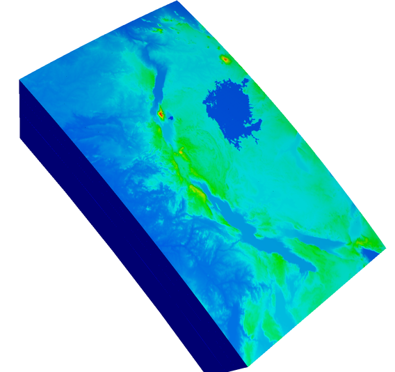
In particular, though you cannot see this here, the top surface is not just colored by the elevation but is, in fact, deformed to follow the correct topography. While the actual application is not relevant here, the geometry is. The domain we are interested in is a part of the Earth that ranges from the surface to a depth of 500km, from 26 to 35 degrees East of the Greenwich meridian, and from 5 degrees North of the equator to 10 degrees South.
This description of the geometry suggests to start with a box \(\hat U=[26,35]\times[-10,5]\times[-500000,0]\) (measured in degrees, degrees, and meters) and to provide a map \(\varphi\) so that \(\varphi^{-1}(\hat U)=\Omega\) where \(\Omega\) is the domain we seek. \((\Omega,\varphi)\) is then a chart, \(\varphi\) the pull-back operator, and \(\varphi^{-1}\) the push-forward operator. If we need a point \(q\) that is the "average" of other points \(q_i\in\Omega\), the ChartManifold class then first applies the pull-back to obtain \(\hat q_i=\varphi(q_i)\), averages these to a point \(\hat p\) and then computes \(p=\varphi^{-1}(\hat p)\).
Our goal here is therefore to implement a class that describes \(\varphi\) and \(\varphi^{-1}\). If Earth was a sphere, then this would not be difficult: if we denote by \((\hat \phi,\hat \theta,\hat d)\) the points of \(\hat U\) (i.e., longitude counted eastward, latitude counted northward, and elevation relative to zero depth), then
\[ \mathbf x = \varphi^{-1}(\hat \phi,\hat \theta,\hat d) = (R+\hat d) (\cos\hat \phi\cos\hat \theta, \sin\hat \phi\cos\hat \theta, \sin\hat \theta)^T \]
provides coordinates in a Cartesian coordinate system, where \(R\) is the radius of the sphere. However, the Earth is not a sphere:
It is flattened at the poles and larger at the equator: the semi-major axis is approximately 22km longer than the semi-minor axis. We will account for this using the WGS 84 reference standard for the Earth shape. The formula used in WGS 84 to obtain a position in Cartesian coordinates from longitude, latitude, and elevation is
\[ \mathbf x = \varphi_\text{WGS84}^{-1}(\phi,\theta,d) = \left( \begin{array}{c} (\bar R(\theta)+d) \cos\phi\cos\theta, \\ (\bar R(\theta)+d) \sin\phi\cos\theta, \\ ((1-e^2)\bar R(\theta)+d) \sin\theta \end{array} \right), \]
where \(\bar R(\theta)=\frac{R}{\sqrt{1-(e \sin\theta)^2}}\), and radius and ellipticity are given by \(R=6378137\text{m}, e=0.081819190842622\). In this formula, we assume that the arguments to sines and cosines are evaluated in degree, not radians (though we will have to change this assumption in the code).
\[ (\phi,\theta,d) = \varphi_\text{topo}^{-1}(\hat\phi,\hat\theta,\hat d) = \left( \hat\phi, \hat\theta, \hat d + \frac{\hat d+500000}{500000}h(\hat\phi,\hat\theta) \right). \]
Using this function, the top surface of the box \(\hat U\) is displaced to the correct topography, the bottom surface remains where it was, and points in between are linearly interpolated.Using these two functions, we can then define the entire push-forward function \(\varphi^{-1}: \hat U \rightarrow \Omega\) as
\[ \mathbf x = \varphi^{-1}(\hat\phi,\hat\theta,\hat d) = \varphi_\text{WGS84}^{-1}(\varphi_\text{topo}^{-1}(\hat\phi,\hat\theta,\hat d)). \]
In addition, we will have to define the inverse of this function, the pull-back operation, which we can write as
\[ (\hat\phi,\hat\theta,\hat d) = \varphi(\mathbf x) = \varphi_\text{topo}(\varphi_\text{WGS84}(\mathbf x)). \]
We can obtain one of the components of this function by inverting the formula above:
\[ (\hat\phi,\hat\theta,\hat d) = \varphi_\text{topo}(\phi,\theta,d) = \left( \phi, \theta, 500000\frac{d-h(\phi,\theta)}{500000+h(\phi,\theta)} \right). \]
Computing \(\varphi_\text{WGS84}(\mathbf x)\) is also possible though a lot more awkward. We won't show the formula here but instead only provide the implementation in the program.
There are a number of issues we need to address in the program. At the largest scale, we need to write a class that implements the interface of ChartManifold. This involves a function push_forward() that takes a point in the reference domain \(\hat U\) and transform it into real space using the function \(\varphi^{-1}\) outlined above, and its inverse function pull_back() implementing \(\varphi\). We will do so in the AfricaGeometry class below that looks, in essence, like this:
The transformations above have two parts: the WGS 84 transformations and the topography transformation. Consequently, the AfricaGeometry class will have additional (non-virtual) member functions AfricaGeometry::push_forward_wgs84() and AfricaGeometry::push_forward_topo() that implement these two pieces, and corresponding pull back functions.
The WGS 84 transformation functions are not particularly interesting (even though the formulas they implement are impressive). The more interesting part is the topography transformation. Recall that for this, we needed to evaluate the elevation function \(h(\hat\phi,\hat\theta)\). There is of course no formula for this: Earth is what it is, the best one can do is look up the altitude from some table. This is, in fact what we will do.
The data we use was originally created by the Shuttle Radar Topography Mission, was downloaded from the US Geologic Survey (USGS) and processed by D. Sarah Stamps who also wrote the initial version of the WGS 84 transformation functions. The topography data so processed is stored in a file topography.txt.gz that, when unpacked looks like this:
The data is formatted as latitude longitude elevation where the first two columns are provided in degrees North of the equator and degrees East of the Greenwich meridian. The final column is given in meters above the WGS 84 zero elevation.
In the transformation functions, we need to evaluate \(h(\hat\phi,\hat\theta)\) for a given longitude \(\hat\phi\) and latitude \(\hat\theta\). In general, this data point will not be available and we will have to interpolate between adjacent data points. Writing such an interpolation routine is not particularly difficult, but it is a bit tedious and error prone. Fortunately, we can somehow shoehorn this data set into an existing class: Functions::InterpolatedUniformGridData . Unfortunately, the class does not fit the bill quite exactly and so we need to work around it a bit. The problem comes from the way we initialize this class: in its simplest form, it takes a stream of values that it assumes form an equispaced mesh in the \(x-y\) plane (or, here, the \(\phi-\theta\) plane). Which is what they do here, sort of: they are ordered latitude first, longitude second; and more awkwardly, the first column starts at the largest values and counts down, rather than the usual other way around.
Now, while tutorial programs are meant to illustrate how to code with deal.II, they do not necessarily have to satisfy the same quality standards as one would have to do with production codes. In a production code, we would write a function that reads the data and (i) automatically determines the extents of the first and second column, (ii) automatically determines the number of data points in each direction, (iii) does the interpolation regardless of the order in which data is arranged, if necessary by switching the order between reading and presenting it to the Functions::InterpolatedUniformGridData class.
On the other hand, tutorial programs are best if they are short and demonstrate key points rather than dwell on unimportant aspects and, thereby, obscure what we really want to show. Consequently, we will allow ourselves a bit of leeway:
All of this then calls for a class that essentially looks like this:
Note how the value() function negates the latitude. It also switches from the format \(\phi,\theta\) that we use everywhere else to the latitude-longitude format used in the table. Finally, it takes its arguments in radians as that is what we do everywhere else in the program, but then converts them to the degree-based system used for table lookup. As you will see in the implementation below, the function has a few more (static) member functions that we will call in the initialization of the topography_data member variable: the class type of this variable has a constructor that allows us to set everything right at construction time, rather than having to fill data later on, but this constructor takes a number of objects that can't be constructed in-place (at least not in C++98). Consequently, the construction of each of the objects we want to pass in the initialization happens in a number of static member functions.
Having discussed the general outline of how we want to implement things, let us go to the program and show how it is done in practice.
Let us start with the include files we need here. Obviously, we need the ones that describe the triangulation (tria.h), and that allow us to create and output triangulations (grid_generator.h and grid_out.h). Furthermore, we need the header file that declares the Manifold and ChartManifold classes that we will need to describe the geometry (manifold.h). We will then also need the GridTools::transform() function from the last of the following header files; the purpose for this function will become discussed at the point where we use it.
The remainder of the include files relate to reading the topography data. As explained in the introduction, we will read it from a file and then use the Functions::InterpolatedUniformGridData class that is declared in the first of the following header files. Because the data is large, the file we read from is stored as gzip compressed data and we make use of some BOOST-provided functionality to read directly from gzipped data.
The last include file is required because we will be using a feature that is not part of the C++11 standard. As some of the C++14 features are very useful, we provide their implementation in an internal namespace, if the compiler does not support them:
The final part of the top matter is to open a namespace into which to put everything, and then to import the dealii namespace into it.
The first significant part of this program is the class that describes the topography \(h(\hat phi,\hat \theta)\) as a function of longitude and latitude. As discussed in the introduction, we will make our life a bit easier here by not writing the class in the most general way possible but by only writing it for the particular purpose we are interested in here: interpolating data obtained from one very specific data file that contains information about a particular area of the world for which we know the extents.
The general layout of the class has been discussed already above. Following is its declaration, including three static member functions that we will need in initializing the topography_data member variable.
Let us move to the implementation of the class. The interesting parts of the class are the constructor and the value() function. The former initializes the Functions::InterpolatedUniformGridData member variable and we will use the constructor that requires us to pass in the end points of the 2-dimensional data set we want to interpolate (which are here given by the intervals \([-6.983333, 11.98333]\), using the trick of switching end points discussed in the introduction, and \([25, 35.983333]\), both given in degrees), the number of intervals into which the data is split (379 in latitude direction and 219 in longitude direction, for a total of \(380\times 220\) data points), and a Table object that contains the data. The data then of course has size \(380\times 220\) and we initialize it by providing an iterator to the first of the 83,600 elements of a std::vector object returned by the get_data() function below. Note that all of the member functions we call here are static because (i) they do not access any member variables of the class, and (ii) because they are called at a time when the object is not initialized fully anyway.
The only other function of greater interest is the get_data() function. It returns a temporary vector that contains all 83,600 data points describing the altitude and is read from the file topography.txt.gz. Because the file is compressed by gzip, we cannot just read it through an object of type std::ifstream, but there are convenient methods in the BOOST library (see http://www.boost.org) that allows us to read from compressed files without first having to uncompress it on disk. The result is, basically, just another input stream that, for all practical purposes, looks just like the ones we always use.
When reading the data, we read the three columns but throw ignore the first two. The datum in the last column is appended to an array that we the return and that will be copied into the table from which topography_data is initialized. Since the BOOST.iostreams library does not provide a very useful exception when the input file does not exist, is not readable, or does not contain the correct number of data lines, we catch all exceptions it may produce and create our own one. To this end, in the catch clause, we let the program run into an AssertThrow(false, ...) statement. Since the condition is always false, this always triggers an exception. In other words, this is equivalent to writing throw ExcMessage("...") but it also fills certain fields in the exception object that will later be printed on the screen identifying the function, file and line where the exception happened.
create a stream where we read from gzipped data
The following class is then the main one of this program. Its structure has been described in much detail in the introduction and does not need much introduction any more.
The implementation, as well, is pretty straightforward if you have read the introduction. In particular, both of the pull back and push forward functions are just concatenations of the respective functions of the WGS 84 and topography mappings:
This function is required by the interface of the Manifold base class, and allows you to clone the AfricaGeometry class. This is where we use a feature that is only available in C++14, namely the make_unique function, that simplifies the creation of std::unique_ptr objects. Notice that, while the function returns an std::unique_ptr<Manifold<3,3> >, we internally create a unique_ptr<AfricaGeometry>. C++11 knows how to handle these cases, and is able to transform a unique pointer to a derived class to a unique pointer to its base class automatically:
The following two functions then define the forward and inverse transformations that correspond to the WGS 84 reference shape of Earth. The forward transform follows the formula shown in the introduction. The inverse transform is significantly more complicated and is, at the very least, not intuitive. It also suffers from the fact that it returns an angle that at the end of the function we need to clip back into the interval \([0,2\pi]\) if it should have escaped from there.
In contrast, the topography transformations follow exactly the description in the introduction. There is not consequently not much to add:
Having so described the properties of the geometry, not it is time to deal with the mesh used to discretize it. To this end, we create objects for the geometry and triangulation, and then proceed to create a \(1\times 2\times 1\) rectangular mesh that corresponds to the reference domain \(\hat U=[26,35]\times[-10,5]\times[-500000,0]\). We choose this number of subdivisions because it leads to cells that are roughly like cubes instead of stretched in one direction or another.
Of course, we are not actually interested in meshing the reference domain. We are interested in meshing the real domain. Consequently, we will use the GridTools::transform() function that simply moves every point of a triangulation according to a given transformation. The transformation function it wants is a function that takes as its single argument a point in the reference domain and returns the corresponding location in the domain that we want to map to. This is, of course, exactly the push forward function of the geometry we use. However, AfricaGeometry::push_forward() requires two arguments: the AfricaGeometry object to work with via its implicit this pointer, and the point. We bind the first of these to the geometry object we have created at the top of the function and leave the second one open, obtaining the desired object to do the transformation.
The next step is to explain to the triangulation to use our geometry object whenever a new point is needed upon refining the mesh. We do this by telling the triangulation to use our geometry for everything that has manifold indicator zero, and then proceed to mark all cells and their bounding faces and edges with manifold indicator zero. This ensures that the triangulation consults our geometry object every time a new vertex is needed. Since manifold indicators are inherited from mother to children, this also happens after several recursive refinement steps.
The last step is to refine the mesh beyond its initial \(1\times 2\times 1\) coarse mesh. We could just refine globally a number of times, but since for the purpose of this tutorial program we're really only interested in what is happening close to the surface, we just refine 6 times all of the cells that have a face at a boundary with indicator 5. Looking this up in the documentation of the GridGenerator::subdivided_hyper_rectangle() function we have used above reveals that boundary indicator 5 corresponds to the top surface of the domain (and this is what the last true argument in the call to GridGenerator::subdivided_hyper_rectangle() above meant: to "color" the boundaries by assigning each boundary a unique boundary indicator).
Having done this all, we can now output the mesh into a file of its own:
Finally, the main function, which follows the same scheme used in all tutorial programs starting with step-6. There isn't much to do here, only to call the single run() function.
Running the program produces a mesh file mesh.vtu that we can visualize with any of the usual visualization programs that can read the VTU file format. If one just looks at the mesh itself, it is actually very difficult to see anything that doesn't just look like a perfectly round piece of a sphere (though if one modified the program so that it does produce a sphere and looked at them at the same time, the difference between the overall sphere and WGS 84 shape is quite apparent). Apparently, Earth is actually quite a flat place. Of course we already know this from satellite pictures. However, we can tease out something more by coloring cells by their volume. This both produces slight variations in hue along the top surface and something for the visualization programs to apply their shading algorithms to (because the top surfaces of the cells are now no longer just tangential to a sphere but tilted):
Yet, at least as far as visualizations are concerned, this is still not too impressive. Rather, let us visualize things in a way so that we show the actual elevation along the top surface. In other words, we want a picture like this, with an incredible amount of detail:
A zoom-in of this picture shows the vertical displacement quite clearly (here, looking from the West-Northwest over the rift valley, the triple peaks of Mount Stanley, Mount Speke, and Mount Baker in the Rwenzori Range, Lake George and toward the great flatness of Lake Victoria):

These image were produced with three small modifications:
An additional seventh mesh refinement towards the top surface for the first of these two pictures, and a total of nine for the second. In the second image, the horizontal mesh size is approximately 1.5km, and just under 1km in vertical direction. (The picture was also created using a more resolved data set; however, it is too big to distribute as part of the tutorial.)
The addition of the following function that, given a point x computes the elevation by converting the point to reference WGS 84 coordinates and only keeping the depth variable (the function is, consequently, a simplified version of the AfricaGeometry::pull_back_wgs84() function):
Adding the following piece to the bottom of the run() function:
This last piece of code first creates a \(Q_1\) finite element space on the mesh. It then (ab)uses VectorTools::interpolate_boundary_values() to evaluate the elevation function for every node at the top boundary (the one with boundary indicator 5). We here wrap the call to get_elevation() with the ScalarFunctionFromFunctionObject class to make a regular C++ function look like an object of a class derived from the Function class that we want to use in VectorTools::interpolate_boundary_values(). Having so gotten a list of degrees of freedom located at the top boundary and corresponding elevation values, we just go down this list and set these elevations in the elevation vector (leaving all interior degrees of freedom at their original zero value). This vector is then output using DataOut as usual and can be visualized as shown above.
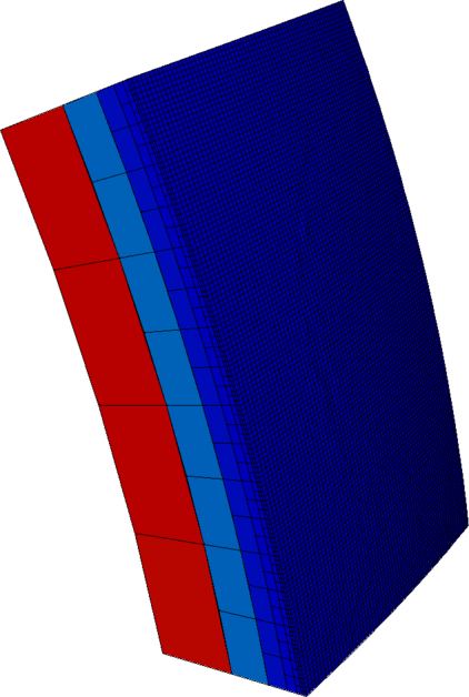
If you zoomed in on the mesh shown above and looked closely enough, you would find that at hanging nodes, the two small edges connecting to the hanging nodes are not in exactly the same location as the large edge of the neighboring cell. This can be shown more clearly by using a different surface description in which we enlarge the vertical topography to enhance the effect (courtesy of Alexander Grayver):

So what is happening here? Partly, this is only a result of visualization, but there is an underlying real cause as well:
When you visualize a mesh using any of the common visualization programs, what they really show you is just a set of edges that are plotted as straight lines in three-dimensional space. This is so because almost all data file formats for visualizing data only describe hexahedral cells as a collection of eight vertices in 3d space, and do not allow to any more complicated descriptions. (This is the main reason why DataOut::build_patches() takes an argument that can be set to something larger than one.) These linear edges may be the edges of the cell you do actual computations on, or they may not, depending on what kind of mapping you use when you do your integrations using FEValues. By default, of course, FEValues uses a linear mapping (i.e., an object of class MappingQ1) and in that case a 3d cell is indeed described exclusively by its 8 vertices and the volume it fills is a trilinear interpolation between these points, resulting in linear edges. But, you could also have used tri-quadratic, tri-cubic, or even higher order mappings and in these cases the volume of each cell will be bounded by quadratic, cubic or higher order polynomial curves. Yet, you only get to see these with linear edges in the visualization program because, as mentioned, file formats do not allow to describe the real geometry of cells.
The situation is slightly more complicated if you use a higher order mapping using the MappingQ class, but not fundamentally different. Let's take a quadratic mapping for the moment (nothing fundamental changes with even higher order mappings). Then you need to imagine each edge of the cells you integrate on as a quadratic curve despite the fact that you will never actually see it plotted that way by a visualization program. But imagine it that way for a second. So which quadratic curve does MappingQ take? It is the quadratic curve that goes through the two vertices at the end of the edge as well as a point in the middle that it queries from the manifold. In the case of the long edge on the unrefined side, that's of course exactly the location of the hanging node, so the quadratic curve describing the long edge does go through the hanging node, unlike in the case of the linear mapping. But the two small edges are also quadratic curves; for example, the left small edge will go through the left vertex of the long edge and the hanging node, plus a point it queries halfway in between from the manifold. Because, as before, the point the manifold returns halfway along the left small edge is rarely exactly on the quadratic curve describing the long edge, the quadratic short edge will typically not coincide with the left half of the quadratic long edge, and the same is true for the right short edge. In other words, again, the geometries of the large cell and its smaller neighbors at hanging nodes do not touch snuggly.
This all begs two questions: first, does it matter, and second, could this be fixed. Let us discuss these in the following:
Does it matter? It is almost certainly true that this depends on the equation you are solving. For example, it is known that solving the Euler equations of gas dynamics on complex geometries requires highly accurate boundary descriptions to ensure convergence of quantities that are measure the flow close to the boundary. On the other hand, equations with elliptic components (e.g., the Laplace or Stokes equations) are typically rather forgiving of these issues: one does quadrature anyway to approximate integrals, and further approximating the geometry may not do as much harm as one could fear given that the volume of the overlaps or gaps at every hanging node is only \({\cal O}(h^d)\) even with a linear mapping and \({\cal O}(h^{d+p-1})\) for a mapping of degree \(p\). (You can see this by considering that in 2d the gap/overlap is a triangle with base \(h\) and height \({\cal O}(h)\); in 3d, it is a pyramid-like structure with base area \(h^2\) and height \({\cal O}(h)\). Similar considerations apply for higher order mappings where the height of the gaps/overlaps is \({\cal O}(h^p)\).) In other words, if you use a linear mapping with linear elements, the error in the volume you integrate over is already at the same level as the integration error using the usual Gauss quadrature. Of course, for higher order elements one would have to choose matching mapping objects.
Another point of view on why it is probably not worth worrying too much about the issue is that there is certainly no narrative in the community of numerical analysts that these issues are a major concern one needs to watch out for when using complex geometries. If it does not seem to be discussed often among practitioners, if ever at all, then it is at least not something people have identified as a common problem.
This issue is not dissimilar to having hanging nodes at curved boundaries where the geometry description of the boundary typically pulls a hanging node onto the boundary whereas the large edge remains straight, making the adjacent small and large cells not match each other. Although this behavior existed in deal.II since its beginning, 15 years before manifold descriptions became available, it did not ever come up in mailing list discussions or conversations with colleagues.
Could it be fixed? In principle, yes, but it's a complicated issue. Let's assume for the moment that we would only ever use the MappingQ1 class, i.e., linear mappings. In that case, whenever the triangulation class requires a new vertex along an edge that would become a hanging node, it would just take the mean value of the adjacent vertices in real space, i.e., without asking the manifold description. This way, the point lies on the long straight edge and the two short straight edges would match the one long edge. Only when all adjacent cells have been refined and the point is no longer a hanging node would we replace its coordinates by coordinates we get by a manifold. This may be awkward to implement, but it would certainly be possible.
The more complicated issue arises because people may want to use a higher order MappingQ object. In that case, the Triangulation class may freely choose the location of the hanging node (because the quadratic curve for the long edge can be chosen in such a way that it goes through the hanging node) but the MappingQ class, when determining the location of mid-edge points must make sure that if the edge is one half of a long edge of a neighboring coarser cell, then the midpoint cannot be obtained from the manifold but must be chosen along the long quadratic edge. For cubic (and all other odd) mappings, the matter is again a bit complicated because one typically arranges the cubic edge to go through points 1/3 and 2/3 along the edge, and thus necessarily through the hanging node, but this could probably be worked out. In any case, even then, there are two problems with this:
Consequently, at least for the moment, none of these ideas are implemented. This leads to the undesirable consequence of discontinuous geometries, but, as discussed above, the effects of this do not appear to pose problem in actual practice.
 1.8.11

