Reference documentation for deal.II version 9.1.0-pre
The step-16 tutorial program

This tutorial depends on step-6.

Table of contents
  1. Introduction
  2. The commented program
  1. Results
  2. The plain program

Introduction

This example shows the basic usage of the multilevel functions in deal.II. It solves almost the same problem as used in step-6, but demonstrating the things one has to provide when using multigrid as a preconditioner. In particular, this requires that we define a hierarchy of levels, provide transfer operators from one level to the next and back, and provide representations of the Laplace operator on each level.

In order to allow sufficient flexibility in conjunction with systems of differential equations and block preconditioners, quite a few different objects have to be created before starting the multilevel method, although most of what needs to be done is provided by deal.II itself. These are

Most of these objects will only be needed inside the function that actually solves the linear system. There, these objects are combined in an object of type Multigrid, containing the implementation of the V-cycle, which is in turn used by the preconditioner PreconditionMG, ready for plug-in into a linear solver of the LAC library.

The multigrid method implemented here for adaptively refined meshes follows the outline in the Multigrid paper, which describes the underlying implementation in deal.II and also introduces a lot of the nomenclature. First, we have to distinguish between level meshes, namely cells that have the same refinement distance from the coarse mesh, and the leaf mesh consisting of active cells of the hierarchy (in older work we refer to this as the global mesh, but this term is overused). Most importantly, the leaf mesh is not identical with the level mesh on the finest level. The following image shows what we consider to be a "level mesh":

multigrid.png

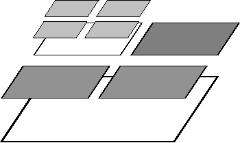
The fine level in this mesh consists only of the degrees of freedom that are defined on the refined cells, but does not extend to that part of the domain that is not refined. While this guarantees that the overall effort grows as \({\cal O}(N)\) as necessary for optimal multigrid complexity, it leads to problems when defining where to smooth and what boundary conditions to pose for the operators defined on individual levels if the level boundary is not an external boundary. These questions are discussed in detail in the article cited above.

The testcase

The problem we solve here is similar to step-6, with two main differences: first, the multigrid preconditioner, obviously. We also change the discontinuity of the coefficients such that the local assembler does not look more complicated than necessary.

The commented program

Include files

Again, the first few include files are already known, so we won't comment on them:

#include <deal.II/base/quadrature_lib.h>
#include <deal.II/base/function.h>
#include <deal.II/base/logstream.h>
#include <deal.II/base/utilities.h>
#include <deal.II/lac/affine_constraints.h>
#include <deal.II/lac/vector.h>
#include <deal.II/lac/full_matrix.h>
#include <deal.II/lac/sparse_matrix.h>
#include <deal.II/lac/solver_cg.h>
#include <deal.II/lac/precondition.h>
#include <deal.II/grid/tria.h>
#include <deal.II/grid/tria_accessor.h>
#include <deal.II/grid/tria_iterator.h>
#include <deal.II/grid/grid_generator.h>
#include <deal.II/grid/grid_refinement.h>
#include <deal.II/dofs/dof_accessor.h>
#include <deal.II/dofs/dof_tools.h>
#include <deal.II/fe/fe_q.h>
#include <deal.II/fe/fe_values.h>
#include <deal.II/numerics/vector_tools.h>
#include <deal.II/numerics/data_out.h>
#include <deal.II/numerics/error_estimator.h>

These, now, are the include necessary for the multilevel methods. The first one declares how to handle Dirichlet boundary conditions on each of the levels of the multigrid method. For the actual description of the degrees of freedom, we do not need any new include file because DoFHandler already has all necessary methods implemented. We will only need to distribute the DoFs for the levels further down.

The rest of the include files deals with the mechanics of multigrid as a linear operator (solver or preconditioner).

#include <deal.II/multigrid/mg_constrained_dofs.h>
#include <deal.II/multigrid/multigrid.h>
#include <deal.II/multigrid/mg_transfer.h>
#include <deal.II/multigrid/mg_tools.h>
#include <deal.II/multigrid/mg_coarse.h>
#include <deal.II/multigrid/mg_smoother.h>
#include <deal.II/multigrid/mg_matrix.h>

Finally we include the MeshWorker framework. This framework through its function loop() and integration_loop(), automates loops over cells and assembling of data into vectors, matrices, etc. It obeys constraints automatically. Since we have to build several matrices and have to be aware of several sets of constraints, this will save us a lot of headache.

#include <deal.II/meshworker/dof_info.h>
#include <deal.II/meshworker/integration_info.h>
#include <deal.II/meshworker/simple.h>
#include <deal.II/meshworker/output.h>
#include <deal.II/meshworker/loop.h>

In order to save effort, we use the pre-implemented Laplacian found in

#include <deal.II/integrators/laplace.h>
#include <deal.II/integrators/l2.h>

This is C++:

#include <iostream>
#include <fstream>
using namespace dealii;
namespace Step16
{

The integrator on each cell

The MeshWorker::integration_loop() expects a class that provides functions for integration on cells and boundary and interior faces. This is done by the following class. In the constructor, we tell the loop that cell integrals should be computed (the 'true'), but integrals should not be computed on boundary and interior faces (the two 'false'). Accordingly, we only need a cell function, but none for the faces.

template <int dim>
class LaplaceIntegrator : public MeshWorker::LocalIntegrator<dim>
{
public:
LaplaceIntegrator();
virtual void cell(MeshWorker::DoFInfo<dim> & dinfo,
MeshWorker::IntegrationInfo<dim> &info) const override;
};
template <int dim>
LaplaceIntegrator<dim>::LaplaceIntegrator()
: MeshWorker::LocalIntegrator<dim>(true, false, false)
{}

Next the actual integrator on each cell. We solve a Poisson problem with a coefficient one in the right half plane and one tenth in the left half plane.

The MeshWorker::LocalResults base class of MeshWorker::DoFInfo contains objects that can be filled in this local integrator. How many objects are created is determined inside the MeshWorker framework by the assembler class. Here, we test for instance that one matrix is required (MeshWorker::LocalResults::n_matrices()). The matrices are accessed through MeshWorker::LocalResults::matrix(), which takes the number of the matrix as its first argument. The second argument is only used for integrals over faces when there are two matrices for each test function used. Then, a second matrix with indicator 'true' would exist with the same index.

MeshWorker::IntegrationInfo provides one or several FEValues objects, which below are used by LocalIntegrators::Laplace::cell_matrix() or LocalIntegrators::L2::L2(). Since we are assembling only a single PDE, there is also only one of these objects with index zero.

In addition, we note that this integrator serves to compute the matrices for the multilevel preconditioner as well as the matrix and the right hand side for the global system. Since the assembler for a system requires an additional vector, MeshWorker::LocalResults::n_vectors() is returning a nonzero value. Accordingly, we fill a right hand side vector at the end of this function. Since LocalResults can deal with several BlockVector objects, but we are again in the simplest case here, we enter the information into block zero of vector zero.

template <int dim>
void
LaplaceIntegrator<dim>::cell(MeshWorker::DoFInfo<dim> & dinfo,
{
const double coefficient = (dinfo.cell->center()(0) > 0.) ? .1 : 1.;
info.fe_values(0),
coefficient);
if (dinfo.n_vectors() > 0)
{
std::vector<double> rhs(info.fe_values(0).n_quadrature_points, 1.);
LocalIntegrators::L2::L2(dinfo.vector(0).block(0),
info.fe_values(0),
rhs);
}
}

The LaplaceProblem class template

This main class is basically the same class as in step-6. As far as member functions is concerned, the only addition is the assemble_multigrid function that assembles the matrices that correspond to the discrete operators on intermediate levels:

template <int dim>
class LaplaceProblem
{
public:
LaplaceProblem(const unsigned int degree);
void run();
private:
void setup_system();
void assemble_system();
void assemble_multigrid();
void solve();
void refine_grid();
void output_results(const unsigned int cycle) const;
Triangulation<dim> triangulation;
DoFHandler<dim> dof_handler;
SparsityPattern sparsity_pattern;
SparseMatrix<double> system_matrix;
Vector<double> solution;
Vector<double> system_rhs;
const unsigned int degree;

The following members are the essential data structures for the multigrid method. The first two represent the sparsity patterns and the matrices on individual levels of the multilevel hierarchy, very much like the objects for the global mesh above.

Then we have two new matrices only needed for multigrid methods with local smoothing on adaptive meshes. They convey data between the interior part of the refined region and the refinement edge, as outlined in detail in the multigrid paper.

The last object stores information about the boundary indices on each level and information about indices lying on a refinement edge between two different refinement levels. It thus serves a similar purpose as AffineConstraints, but on each level.

MGLevelObject<SparsityPattern> mg_sparsity_patterns;
MGConstrainedDoFs mg_constrained_dofs;
};

The LaplaceProblem class implementation

Just one short remark about the constructor of the Triangulation: by convention, all adaptively refined triangulations in deal.II never change by more than one level across a face between cells. For our multigrid algorithms, however, we need a slightly stricter guarantee, namely that the mesh also does not change by more than refinement level across vertices that might connect two cells. In other words, we must prevent the following situation:

limit_level_difference_at_vertices.png

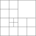
This is achieved by passing the Triangulation::limit_level_difference_at_vertices flag to the constructor of the triangulation class.

template <int dim>
LaplaceProblem<dim>::LaplaceProblem(const unsigned int degree)
: triangulation(Triangulation<dim>::limit_level_difference_at_vertices)
, fe(degree)
, dof_handler(triangulation)
, degree(degree)
{}

LaplaceProblem::setup_system

In addition to just distributing the degrees of freedom in the DoFHandler, we do the same on each level. Then, we follow the same procedure as before to set up the system on the leaf mesh.

template <int dim>
void LaplaceProblem<dim>::setup_system()
{
dof_handler.distribute_dofs(fe);
dof_handler.distribute_mg_dofs();
deallog << " Number of degrees of freedom: " << dof_handler.n_dofs()
<< " (by level: ";
for (unsigned int level = 0; level < triangulation.n_levels(); ++level)
deallog << dof_handler.n_dofs(level)
<< (level == triangulation.n_levels() - 1 ? ")" : ", ");
deallog << std::endl;
DynamicSparsityPattern dsp(dof_handler.n_dofs(), dof_handler.n_dofs());
solution.reinit(dof_handler.n_dofs());
system_rhs.reinit(dof_handler.n_dofs());
constraints.clear();
DoFTools::make_hanging_node_constraints(dof_handler, constraints);
std::set<types::boundary_id> dirichlet_boundary_ids = {0};
Functions::ZeroFunction<dim> homogeneous_dirichlet_bc;
const std::map<types::boundary_id, const Function<dim> *>
dirichlet_boundary_functions = {
{types::boundary_id(0), &homogeneous_dirichlet_bc}};
static_cast<const DoFHandler<dim> &>(dof_handler),
dirichlet_boundary_functions,
constraints);
constraints.close();
constraints.condense(dsp);
sparsity_pattern.copy_from(dsp);
system_matrix.reinit(sparsity_pattern);

The multigrid constraints have to be initialized. They need to know about the boundary values as well, so we pass the dirichlet_boundary here as well.

mg_constrained_dofs.clear();
mg_constrained_dofs.initialize(dof_handler);
mg_constrained_dofs.make_zero_boundary_constraints(dof_handler,
dirichlet_boundary_ids);

Now for the things that concern the multigrid data structures. First, we resize the multilevel objects to hold matrices and sparsity patterns for every level. The coarse level is zero (this is mandatory right now but may change in a future revision). Note that these functions take a complete, inclusive range here (not a starting index and size), so the finest level is n_levels-1. We first have to resize the container holding the SparseMatrix classes, since they have to release their SparsityPattern before the can be destroyed upon resizing.

const unsigned int n_levels = triangulation.n_levels();
mg_interface_in.resize(0, n_levels - 1);
mg_interface_in.clear_elements();
mg_interface_out.resize(0, n_levels - 1);
mg_interface_out.clear_elements();
mg_matrices.resize(0, n_levels - 1);
mg_matrices.clear_elements();
mg_sparsity_patterns.resize(0, n_levels - 1);

Now, we have to provide a matrix on each level. To this end, we first use the MGTools::make_sparsity_pattern function to generate a preliminary compressed sparsity pattern on each level (see the Sparsity patterns module for more information on this topic) and then copy it over to the one we really want. The next step is to initialize both kinds of level matrices with these sparsity patterns.

It may be worth pointing out that the interface matrices only have entries for degrees of freedom that sit at or next to the interface between coarser and finer levels of the mesh. They are therefore even sparser than the matrices on the individual levels of our multigrid hierarchy. If we were more concerned about memory usage (and possibly the speed with which we can multiply with these matrices), we should use separate and different sparsity patterns for these two kinds of matrices.

for (unsigned int level = 0; level < n_levels; ++level)
{
DynamicSparsityPattern dsp(dof_handler.n_dofs(level),
dof_handler.n_dofs(level));
MGTools::make_sparsity_pattern(dof_handler, dsp, level);
mg_sparsity_patterns[level].copy_from(dsp);
mg_matrices[level].reinit(mg_sparsity_patterns[level]);
mg_interface_in[level].reinit(mg_sparsity_patterns[level]);
mg_interface_out[level].reinit(mg_sparsity_patterns[level]);
}
}

LaplaceProblem::assemble_system

The following function assembles the linear system on the finest level of the mesh. Since we want to reuse the code here for the level assembling below, we use the local integrator class LaplaceIntegrator and leave the loops to the MeshWorker framework. Thus, this function first sets up the objects necessary for this framework, namely

After the loop has combined all of these into a matrix and a right hand side, there is one thing left to do: the assemblers leave matrix rows and columns of constrained degrees of freedom untouched. Therefore, we put a one on the diagonal to make the whole system well posed. The value one, or any fixed value has the advantage, that its effect on the spectrum of the matrix is easily understood. Since the corresponding eigenvectors form an invariant subspace, the value chosen does not affect the convergence of Krylov space solvers.

template <int dim>
void LaplaceProblem<dim>::assemble_system()
{
MappingQ1<dim> mapping;
UpdateFlags update_flags =
info_box.add_update_flags_all(update_flags);
info_box.initialize(fe, mapping);
MeshWorker::DoFInfo<dim> dof_info(dof_handler);
assembler;
assembler.initialize(constraints);
assembler.initialize(system_matrix, system_rhs);
LaplaceIntegrator<dim> matrix_integrator;
MeshWorker::integration_loop<dim, dim>(dof_handler.begin_active(),
dof_handler.end(),
dof_info,
info_box,
matrix_integrator,
assembler);
for (unsigned int i = 0; i < dof_handler.n_dofs(); ++i)
if (constraints.is_constrained(i))
system_matrix.set(i, i, 1.);
}

LaplaceProblem::assemble_multigrid

The next function is the one that builds the linear operators (matrices) that define the multigrid method on each level of the mesh. The integration core is the same as above, but the loop below will go over all existing cells instead of just the active ones, and the results must be entered into the correct level matrices. Fortunately, MeshWorker hides most of that from us, and thus the difference between this function and the previous lies only in the setup of the assembler and the different iterators in the loop. Also, fixing up the matrices in the end is a little more complicated.

template <int dim>
void LaplaceProblem<dim>::assemble_multigrid()
{
MappingQ1<dim> mapping;
UpdateFlags update_flags =
info_box.add_update_flags_all(update_flags);
info_box.initialize(fe, mapping);
MeshWorker::DoFInfo<dim> dof_info(dof_handler);
assembler.initialize(mg_constrained_dofs);
assembler.initialize(mg_matrices);
assembler.initialize_interfaces(mg_interface_in, mg_interface_out);
LaplaceIntegrator<dim> matrix_integrator;
MeshWorker::integration_loop<dim, dim>(dof_handler.begin_mg(),
dof_handler.end_mg(),
dof_info,
info_box,
matrix_integrator,
assembler);
const unsigned int nlevels = triangulation.n_levels();
for (unsigned int level = 0; level < nlevels; ++level)
{
for (unsigned int i = 0; i < dof_handler.n_dofs(level); ++i)
if (mg_constrained_dofs.is_boundary_index(level, i) ||
mg_constrained_dofs.at_refinement_edge(level, i))
mg_matrices[level].set(i, i, 1.);
}
}

LaplaceProblem::solve

This is the other function that is significantly different in support of the multigrid solver (or, in fact, the preconditioner for which we use the multigrid method).

Let us start out by setting up two of the components of multilevel methods: transfer operators between levels, and a solver on the coarsest level. In finite element methods, the transfer operators are derived from the finite element function spaces involved and can often be computed in a generic way independent of the problem under consideration. In that case, we can use the MGTransferPrebuilt class that, given the constraints of the final linear system and the MGConstrainedDoFs object that knows about the boundary conditions on the each level and the degrees of freedom on interfaces between different refinement level can build the matrices for those transfer operations from a DoFHandler object with level degrees of freedom.

The second part of the following lines deals with the coarse grid solver. Since our coarse grid is very coarse indeed, we decide for a direct solver (a Householder decomposition of the coarsest level matrix), even if its implementation is not particularly sophisticated. If our coarse mesh had many more cells than the five we have here, something better suited would obviously be necessary here.

template <int dim>
void LaplaceProblem<dim>::solve()
{
MGTransferPrebuilt<Vector<double>> mg_transfer(mg_constrained_dofs);
mg_transfer.build_matrices(dof_handler);
FullMatrix<double> coarse_matrix;
coarse_matrix.copy_from(mg_matrices[0]);
MGCoarseGridHouseholder<> coarse_grid_solver;
coarse_grid_solver.initialize(coarse_matrix);

The next component of a multilevel solver or preconditioner is that we need a smoother on each level. A common choice for this is to use the application of a relaxation method (such as the SOR, Jacobi or Richardson method) or a small number of iterations of a solver method (such as CG or GMRES). The mg::SmootherRelaxation and MGSmootherPrecondition classes provide support for these two kinds of smoothers. Here, we opt for the application of a single SOR iteration. To this end, we define an appropriate alias and then setup a smoother object.

The last step is to initialize the smoother object with our level matrices and to set some smoothing parameters. The initialize() function can optionally take additional arguments that will be passed to the smoother object on each level. In the current case for the SOR smoother, this could, for example, include a relaxation parameter. However, we here leave these at their default values. The call to set_steps() indicates that we will use two pre- and two post-smoothing steps on each level; to use a variable number of smoother steps on different levels, more options can be set in the constructor call to the mg_smoother object.

The last step results from the fact that we use the SOR method as a smoother - which is not symmetric - but we use the conjugate gradient iteration (which requires a symmetric preconditioner) below, we need to let the multilevel preconditioner make sure that we get a symmetric operator even for nonsymmetric smoothers:

mg_smoother.initialize(mg_matrices);
mg_smoother.set_steps(2);
mg_smoother.set_symmetric(true);

The next preparatory step is that we must wrap our level and interface matrices in an object having the required multiplication functions. We will create two objects for the interface objects going from coarse to fine and the other way around; the multigrid algorithm will later use the transpose operator for the latter operation, allowing us to initialize both up and down versions of the operator with the matrices we already built:

mg::Matrix<Vector<double>> mg_matrix(mg_matrices);
mg::Matrix<Vector<double>> mg_interface_up(mg_interface_in);
mg::Matrix<Vector<double>> mg_interface_down(mg_interface_out);

Now, we are ready to set up the V-cycle operator and the multilevel preconditioner.

mg_matrix, coarse_grid_solver, mg_transfer, mg_smoother, mg_smoother);
mg.set_edge_matrices(mg_interface_down, mg_interface_up);
preconditioner(dof_handler, mg, mg_transfer);

With all this together, we can finally get about solving the linear system in the usual way:

SolverControl solver_control(1000, 1e-12);
SolverCG<> solver(solver_control);
solution = 0;
solver.solve(system_matrix, solution, system_rhs, preconditioner);
constraints.distribute(solution);
}

Postprocessing

The following two functions postprocess a solution once it is computed. In particular, the first one refines the mesh at the beginning of each cycle while the second one outputs results at the end of each such cycle. The functions are almost unchanged from those in step-6, with the exception of one minor difference: we generate output in VTK format, to use the more modern visualization programs available today compared to those that were available when step-6 was written.

template <int dim>
void LaplaceProblem<dim>::refine_grid()
{
Vector<float> estimated_error_per_cell(triangulation.n_active_cells());
dof_handler,
std::map<types::boundary_id, const Function<dim> *>(),
solution,
estimated_error_per_cell);
estimated_error_per_cell,
0.3,
0.03);
triangulation.execute_coarsening_and_refinement();
}
template <int dim>
void LaplaceProblem<dim>::output_results(const unsigned int cycle) const
{
DataOut<dim> data_out;
data_out.attach_dof_handler(dof_handler);
data_out.add_data_vector(solution, "solution");
data_out.build_patches();
std::ofstream output("solution-" + std::to_string(cycle) + ".vtk");
data_out.write_vtk(output);
}

LaplaceProblem::run

Like several of the functions above, this is almost exactly a copy of the corresponding function in step-6. The only difference is the call to assemble_multigrid that takes care of forming the matrices on every level that we need in the multigrid method.

template <int dim>
void LaplaceProblem<dim>::run()
{
for (unsigned int cycle = 0; cycle < 8; ++cycle)
{
deallog << "Cycle " << cycle << std::endl;
if (cycle == 0)
{
GridGenerator::hyper_ball(triangulation);
triangulation.refine_global(1);
}
else
refine_grid();
deallog << " Number of active cells: "
<< triangulation.n_active_cells() << std::endl;
setup_system();
assemble_system();
assemble_multigrid();
solve();
output_results(cycle);
}
}
} // namespace Step16

The main() function

This is again the same function as in step-6:

int main()
{
try
{
using namespace Step16;
deallog.depth_console(2);
LaplaceProblem<2> laplace_problem(1);
laplace_problem.run();
}
catch (std::exception &exc)
{
std::cerr << std::endl
<< std::endl
<< "----------------------------------------------------"
<< std::endl;
std::cerr << "Exception on processing: " << std::endl
<< exc.what() << std::endl
<< "Aborting!" << std::endl
<< "----------------------------------------------------"
<< std::endl;
return 1;
}
catch (...)
{
std::cerr << std::endl
<< std::endl
<< "----------------------------------------------------"
<< std::endl;
std::cerr << "Unknown exception!" << std::endl
<< "Aborting!" << std::endl
<< "----------------------------------------------------"
<< std::endl;
return 1;
}
return 0;
}

Results

On the finest mesh, the solution looks like this:

More importantly, we would like to see if the multigrid method really improved the solver performance. Therefore, here is the textual output:

DEAL::Cycle 0
DEAL::   Number of active cells:       20
DEAL::   Number of degrees of freedom: 25 (by level: 8, 25)
DEAL:cg::Starting value 0.510691
DEAL:cg::Convergence step 6 value 4.59193e-14
DEAL::Cycle 1
DEAL::   Number of active cells:       41
DEAL::   Number of degrees of freedom: 52 (by level: 8, 25, 41)
DEAL:cg::Starting value 0.455356
DEAL:cg::Convergence step 8 value 3.09682e-13
DEAL::Cycle 2
DEAL::   Number of active cells:       80
DEAL::   Number of degrees of freedom: 100 (by level: 8, 25, 61, 52)
DEAL:cg::Starting value 0.394469
DEAL:cg::Convergence step 9 value 1.96993e-13
DEAL::Cycle 3
DEAL::   Number of active cells:       161
DEAL::   Number of degrees of freedom: 190 (by level: 8, 25, 77, 160)
DEAL:cg::Starting value 0.322156
DEAL:cg::Convergence step 9 value 2.94418e-13
DEAL::Cycle 4
DEAL::   Number of active cells:       311
DEAL::   Number of degrees of freedom: 364 (by level: 8, 25, 86, 227, 174)
DEAL:cg::Starting value 0.279667
DEAL:cg::Convergence step 10 value 3.45746e-13
DEAL::Cycle 5
DEAL::   Number of active cells:       593
DEAL::   Number of degrees of freedom: 667 (by level: 8, 25, 89, 231, 490, 96)
DEAL:cg::Starting value 0.215917
DEAL:cg::Convergence step 10 value 1.03758e-13
DEAL::Cycle 6
DEAL::   Number of active cells:       1127
DEAL::   Number of degrees of freedom: 1251 (by level: 8, 25, 89, 274, 760, 417, 178)
DEAL:cg::Starting value 0.185906
DEAL:cg::Convergence step 10 value 3.40351e-13
DEAL::Cycle 7
DEAL::   Number of active cells:       2144
DEAL::   Number of degrees of freedom: 2359 (by level: 8, 25, 89, 308, 779, 1262, 817)
DEAL:cg::Starting value 0.141519
DEAL:cg::Convergence step 10 value 5.74965e-13

That's almost perfect multigrid performance: 12 orders of magnitude in 10 iteration steps, and almost independent of the mesh size. That's obviously in part due to the simple nature of the problem solved, but it shows the power of multigrid methods.

Possible extensions

We encourage you to switch on timing output by calling the function LogStream::log_execution_time() of the deallog object and compare to step 6. You will see that the multigrid method has quite an overhead on coarse meshes, but that it always beats other methods on fine meshes because of its optimal complexity.

A close inspection of this program's performance shows that it is mostly dominated by matrix-vector operations. step-37 shows one way how this can be avoided by working with matrix-free methods.

Another avenue would be to use algebraic multigrid methods. The geometric multigrid method used here can at times be a bit awkward to implement because it needs all those additional data structures, and it becomes even more difficult if the program is to run in parallel on machines coupled through MPI, for example. In that case, it would be simpler if one could use a black-box preconditioner that uses some sort of multigrid hierarchy for good performance but can figure out level matrices and similar things by itself. Algebraic multigrid methods do exactly this, and we will use them in step-31 for the solution of a Stokes problemm and in step-32 and step-40 for a parallel variation.

Finally, one may want to think how to use geometric multigrid for other kinds of problems, specifically vector valued problems. This is the topic of step-56 where we use the techniques shown here for the Stokes equation.

The plain program

/* ---------------------------------------------------------------------
*
* Copyright (C) 2003 - 2018 by the deal.II authors
*
* This file is part of the deal.II library.
*
* The deal.II library is free software; you can use it, redistribute
* it, and/or modify it under the terms of the GNU Lesser General
* Public License as published by the Free Software Foundation; either
* version 2.1 of the License, or (at your option) any later version.
* The full text of the license can be found in the file LICENSE.md at
* the top level directory of deal.II.
*
* ---------------------------------------------------------------------
*
* Authors: Guido Kanschat, University of Heidelberg, 2003
* Baerbel Janssen, University of Heidelberg, 2010
* Wolfgang Bangerth, Texas A&M University, 2010
*/
#include <deal.II/base/quadrature_lib.h>
#include <deal.II/base/function.h>
#include <deal.II/base/logstream.h>
#include <deal.II/base/utilities.h>
#include <deal.II/lac/affine_constraints.h>
#include <deal.II/lac/vector.h>
#include <deal.II/lac/full_matrix.h>
#include <deal.II/lac/sparse_matrix.h>
#include <deal.II/lac/solver_cg.h>
#include <deal.II/lac/precondition.h>
#include <deal.II/grid/tria.h>
#include <deal.II/grid/tria_accessor.h>
#include <deal.II/grid/tria_iterator.h>
#include <deal.II/grid/grid_generator.h>
#include <deal.II/grid/grid_refinement.h>
#include <deal.II/dofs/dof_accessor.h>
#include <deal.II/dofs/dof_tools.h>
#include <deal.II/fe/fe_q.h>
#include <deal.II/fe/fe_values.h>
#include <deal.II/numerics/vector_tools.h>
#include <deal.II/numerics/data_out.h>
#include <deal.II/numerics/error_estimator.h>
#include <deal.II/multigrid/mg_constrained_dofs.h>
#include <deal.II/multigrid/multigrid.h>
#include <deal.II/multigrid/mg_transfer.h>
#include <deal.II/multigrid/mg_tools.h>
#include <deal.II/multigrid/mg_coarse.h>
#include <deal.II/multigrid/mg_smoother.h>
#include <deal.II/multigrid/mg_matrix.h>
#include <deal.II/meshworker/dof_info.h>
#include <deal.II/meshworker/integration_info.h>
#include <deal.II/meshworker/simple.h>
#include <deal.II/meshworker/output.h>
#include <deal.II/meshworker/loop.h>
#include <deal.II/integrators/laplace.h>
#include <deal.II/integrators/l2.h>
#include <iostream>
#include <fstream>
using namespace dealii;
namespace Step16
{
template <int dim>
class LaplaceIntegrator : public MeshWorker::LocalIntegrator<dim>
{
public:
LaplaceIntegrator();
virtual void cell(MeshWorker::DoFInfo<dim> & dinfo,
MeshWorker::IntegrationInfo<dim> &info) const override;
};
template <int dim>
LaplaceIntegrator<dim>::LaplaceIntegrator()
: MeshWorker::LocalIntegrator<dim>(true, false, false)
{}
template <int dim>
void
LaplaceIntegrator<dim>::cell(MeshWorker::DoFInfo<dim> & dinfo,
{
const double coefficient = (dinfo.cell->center()(0) > 0.) ? .1 : 1.;
info.fe_values(0),
coefficient);
if (dinfo.n_vectors() > 0)
{
std::vector<double> rhs(info.fe_values(0).n_quadrature_points, 1.);
LocalIntegrators::L2::L2(dinfo.vector(0).block(0),
info.fe_values(0),
rhs);
}
}
template <int dim>
class LaplaceProblem
{
public:
LaplaceProblem(const unsigned int degree);
void run();
private:
void setup_system();
void assemble_system();
void assemble_multigrid();
void solve();
void refine_grid();
void output_results(const unsigned int cycle) const;
Triangulation<dim> triangulation;
DoFHandler<dim> dof_handler;
SparsityPattern sparsity_pattern;
SparseMatrix<double> system_matrix;
Vector<double> system_rhs;
const unsigned int degree;
MGLevelObject<SparsityPattern> mg_sparsity_patterns;
MGConstrainedDoFs mg_constrained_dofs;
};
template <int dim>
LaplaceProblem<dim>::LaplaceProblem(const unsigned int degree)
: triangulation(Triangulation<dim>::limit_level_difference_at_vertices)
, fe(degree)
, dof_handler(triangulation)
, degree(degree)
{}
template <int dim>
void LaplaceProblem<dim>::setup_system()
{
dof_handler.distribute_dofs(fe);
dof_handler.distribute_mg_dofs();
deallog << " Number of degrees of freedom: " << dof_handler.n_dofs()
<< " (by level: ";
for (unsigned int level = 0; level < triangulation.n_levels(); ++level)
deallog << dof_handler.n_dofs(level)
<< (level == triangulation.n_levels() - 1 ? ")" : ", ");
deallog << std::endl;
DynamicSparsityPattern dsp(dof_handler.n_dofs(), dof_handler.n_dofs());
solution.reinit(dof_handler.n_dofs());
system_rhs.reinit(dof_handler.n_dofs());
constraints.clear();
DoFTools::make_hanging_node_constraints(dof_handler, constraints);
std::set<types::boundary_id> dirichlet_boundary_ids = {0};
Functions::ZeroFunction<dim> homogeneous_dirichlet_bc;
const std::map<types::boundary_id, const Function<dim> *>
dirichlet_boundary_functions = {
{types::boundary_id(0), &homogeneous_dirichlet_bc}};
static_cast<const DoFHandler<dim> &>(dof_handler),
dirichlet_boundary_functions,
constraints);
constraints.close();
constraints.condense(dsp);
sparsity_pattern.copy_from(dsp);
system_matrix.reinit(sparsity_pattern);
mg_constrained_dofs.clear();
mg_constrained_dofs.initialize(dof_handler);
mg_constrained_dofs.make_zero_boundary_constraints(dof_handler,
dirichlet_boundary_ids);
const unsigned int n_levels = triangulation.n_levels();
mg_interface_in.resize(0, n_levels - 1);
mg_interface_in.clear_elements();
mg_interface_out.resize(0, n_levels - 1);
mg_interface_out.clear_elements();
mg_matrices.resize(0, n_levels - 1);
mg_matrices.clear_elements();
mg_sparsity_patterns.resize(0, n_levels - 1);
for (unsigned int level = 0; level < n_levels; ++level)
{
DynamicSparsityPattern dsp(dof_handler.n_dofs(level),
dof_handler.n_dofs(level));
MGTools::make_sparsity_pattern(dof_handler, dsp, level);
mg_sparsity_patterns[level].copy_from(dsp);
mg_matrices[level].reinit(mg_sparsity_patterns[level]);
mg_interface_in[level].reinit(mg_sparsity_patterns[level]);
mg_interface_out[level].reinit(mg_sparsity_patterns[level]);
}
}
template <int dim>
void LaplaceProblem<dim>::assemble_system()
{
MappingQ1<dim> mapping;
UpdateFlags update_flags =
info_box.add_update_flags_all(update_flags);
info_box.initialize(fe, mapping);
MeshWorker::DoFInfo<dim> dof_info(dof_handler);
assembler;
assembler.initialize(constraints);
assembler.initialize(system_matrix, system_rhs);
LaplaceIntegrator<dim> matrix_integrator;
MeshWorker::integration_loop<dim, dim>(dof_handler.begin_active(),
dof_handler.end(),
dof_info,
info_box,
matrix_integrator,
assembler);
for (unsigned int i = 0; i < dof_handler.n_dofs(); ++i)
if (constraints.is_constrained(i))
system_matrix.set(i, i, 1.);
}
template <int dim>
void LaplaceProblem<dim>::assemble_multigrid()
{
MappingQ1<dim> mapping;
UpdateFlags update_flags =
info_box.add_update_flags_all(update_flags);
info_box.initialize(fe, mapping);
MeshWorker::DoFInfo<dim> dof_info(dof_handler);
assembler.initialize(mg_constrained_dofs);
assembler.initialize(mg_matrices);
assembler.initialize_interfaces(mg_interface_in, mg_interface_out);
LaplaceIntegrator<dim> matrix_integrator;
MeshWorker::integration_loop<dim, dim>(dof_handler.begin_mg(),
dof_handler.end_mg(),
dof_info,
info_box,
matrix_integrator,
assembler);
const unsigned int nlevels = triangulation.n_levels();
for (unsigned int level = 0; level < nlevels; ++level)
{
for (unsigned int i = 0; i < dof_handler.n_dofs(level); ++i)
if (mg_constrained_dofs.is_boundary_index(level, i) ||
mg_constrained_dofs.at_refinement_edge(level, i))
mg_matrices[level].set(i, i, 1.);
}
}
template <int dim>
void LaplaceProblem<dim>::solve()
{
MGTransferPrebuilt<Vector<double>> mg_transfer(mg_constrained_dofs);
mg_transfer.build_matrices(dof_handler);
FullMatrix<double> coarse_matrix;
coarse_matrix.copy_from(mg_matrices[0]);
MGCoarseGridHouseholder<> coarse_grid_solver;
coarse_grid_solver.initialize(coarse_matrix);
mg_smoother.initialize(mg_matrices);
mg_smoother.set_steps(2);
mg_smoother.set_symmetric(true);
mg::Matrix<Vector<double>> mg_matrix(mg_matrices);
mg::Matrix<Vector<double>> mg_interface_up(mg_interface_in);
mg::Matrix<Vector<double>> mg_interface_down(mg_interface_out);
mg_matrix, coarse_grid_solver, mg_transfer, mg_smoother, mg_smoother);
mg.set_edge_matrices(mg_interface_down, mg_interface_up);
preconditioner(dof_handler, mg, mg_transfer);
SolverControl solver_control(1000, 1e-12);
SolverCG<> solver(solver_control);
solution = 0;
solver.solve(system_matrix, solution, system_rhs, preconditioner);
constraints.distribute(solution);
}
template <int dim>
void LaplaceProblem<dim>::refine_grid()
{
Vector<float> estimated_error_per_cell(triangulation.n_active_cells());
dof_handler,
std::map<types::boundary_id, const Function<dim> *>(),
solution,
estimated_error_per_cell);
estimated_error_per_cell,
0.3,
0.03);
triangulation.execute_coarsening_and_refinement();
}
template <int dim>
void LaplaceProblem<dim>::output_results(const unsigned int cycle) const
{
DataOut<dim> data_out;
data_out.attach_dof_handler(dof_handler);
data_out.add_data_vector(solution, "solution");
data_out.build_patches();
std::ofstream output("solution-" + std::to_string(cycle) + ".vtk");
data_out.write_vtk(output);
}
template <int dim>
void LaplaceProblem<dim>::run()
{
for (unsigned int cycle = 0; cycle < 8; ++cycle)
{
deallog << "Cycle " << cycle << std::endl;
if (cycle == 0)
{
GridGenerator::hyper_ball(triangulation);
triangulation.refine_global(1);
}
else
refine_grid();
deallog << " Number of active cells: "
<< triangulation.n_active_cells() << std::endl;
setup_system();
assemble_system();
assemble_multigrid();
solve();
output_results(cycle);
}
}
} // namespace Step16
int main()
{
try
{
using namespace Step16;
deallog.depth_console(2);
LaplaceProblem<2> laplace_problem(1);
laplace_problem.run();
}
catch (std::exception &exc)
{
std::cerr << std::endl
<< std::endl
<< "----------------------------------------------------"
<< std::endl;
std::cerr << "Exception on processing: " << std::endl
<< exc.what() << std::endl
<< "Aborting!" << std::endl
<< "----------------------------------------------------"
<< std::endl;
return 1;
}
catch (...)
{
std::cerr << std::endl
<< std::endl
<< "----------------------------------------------------"
<< std::endl;
std::cerr << "Unknown exception!" << std::endl
<< "Aborting!" << std::endl
<< "----------------------------------------------------"
<< std::endl;
return 1;
}
return 0;
}