|
Reference documentation for deal.II version 9.1.0-pre
|
|
Reference documentation for deal.II version 9.1.0-pre
|
This tutorial depends on step-3.
| Table of contents | |
|---|---|
deal.II has a unique feature which we call ``dimension independent programming''. You may have noticed in the previous examples that many classes had a number in angle brackets suffixed to them. This is to indicate that for example the triangulation in two and three space dimensions are different, but related data types. We could as well have called them Triangulation2d and Triangulation3d instead of Triangulation<2> and Triangulation<3> to name the two classes, but this has an important drawback: assume you have a function which does exactly the same functionality, but on 2d or 3d triangulations, depending on which dimension we would like to solve the equation in presently (if you don't believe that it is the common case that a function does something that is the same in all dimensions, just take a look at the code below - there are almost no distinctions between 2d and 3d!). We would have to write the same function twice, once working on Triangulation2d and once working with a Triangulation3d. This is an unnecessary obstacle in programming and leads to a nuisance to keep the two function in sync (at best) or difficult to find errors if the two versions get out of sync (at worst; this would probably the more common case).
Such obstacles can be circumvented by using some template magic as provided by the C++ language: templatized classes and functions are not really classes or functions but only a pattern depending on an as-yet undefined data type parameter or on a numerical value which is also unknown at the point of definition. However, the compiler can build proper classes or functions from these templates if you provide it with the information that is needed for that. Of course, parts of the template can depend on the template parameters, and they will be resolved at the time of compilation for a specific template parameter. For example, consider the following piece of code:
At the point where the compiler sees this function, it does not know anything about the actual value of dim. The only thing the compiler has is a template, i.e. a blueprint, to generate functions make_grid if given a particular value of dim. Since dim has an unknown value, there is no code the compiler can generate for the moment.
However, if later down the compiler would encounter code that looks, for example, like this,
then the compiler will deduce that the function make_grid for dim==2 was requested and will compile the template above into a function with dim replaced by 2 everywhere, i.e. it will compile the function as if it were defined as
However, it is worth to note that the function GridGenerator::hyper_cube depends on the dimension as well, so in this case, the compiler will call the function GridGenerator::hyper_cube<2> while if dim were 3, it would call GridGenerator::hyper_cube<3> which might be (and actually is) a totally unrelated function.
The same can be done with member variables. Consider the following function, which might in turn call the above one:
This function has a member variable of type DoFHandler<dim>. Again, the compiler can't compile this function until it knows for which dimension. If you call this function for a specific dimension as above, the compiler will take the template, replace all occurrences of dim by the dimension for which it was called, and compile it. If you call the function several times for different dimensions, it will compile it several times, each time calling the right make_grid function and reserving the right amount of memory for the member variable; note that the size of a DoFHandler might, and indeed does, depend on the space dimension.
The deal.II library is build around this concept of dimension-independent programming, and therefore allows you to program in a way that will not need to distinguish between the space dimensions. It should be noted that in only a very few places is it necessary to actually compare the dimension using ifs or switches. However, since the compiler has to compile each function for each dimension separately, even there it knows the value of dim at the time of compilation and will therefore be able to optimize away the if statement along with the unused branch.
In this example program, we will show how to program dimension independently (which in fact is even simpler than if you had to take care about the dimension) and we will extend the Laplace problem of the last example to a program that runs in two and three space dimensions at the same time. Other extensions are the use of a non-constant right hand side function and of non-zero boundary values.
typename in so many places. If you are not entirely familiar with this already, then several of these difficulties are explained in the deal.II Frequently Asked Questions (FAQ) linked to from the deal.II homepage.The first few (many?) include files have already been used in the previous example, so we will not explain their meaning here again.
This is new, however: in the previous example we got some unwanted output from the linear solvers. If we want to suppress it, we have to include this file and add a single line somewhere to the program (see the main() function below for that):
The final step, as in previous programs, is to import all the deal.II class and function names into the global namespace:
Step4 class templateThis is again the same Step4 class as in the previous example. The only difference is that we have now declared it as a class with a template parameter, and the template parameter is of course the spatial dimension in which we would like to solve the Laplace equation. Of course, several of the member variables depend on this dimension as well, in particular the Triangulation class, which has to represent quadrilaterals or hexahedra, respectively. Apart from this, everything is as before.
In the following, we declare two more classes denoting the right hand side and the non-homogeneous Dirichlet boundary values. Both are functions of a dim-dimensional space variable, so we declare them as templates as well.
Each of these classes is derived from a common, abstract base class Function, which declares the common interface which all functions have to follow. In particular, concrete classes have to overload the value function, which takes a point in dim-dimensional space as parameters and shall return the value at that point as a double variable.
The value function takes a second argument, which we have here named component: This is only meant for vector valued functions, where you may want to access a certain component of the vector at the point p. However, our functions are scalar, so we need not worry about this parameter and we will not use it in the implementation of the functions. Inside the library's header files, the Function base class's declaration of the value function has a default value of zero for the component, so we will access the value function of the right hand side with only one parameter, namely the point where we want to evaluate the function. A value for the component can then simply be omitted for scalar functions.
Function objects are used in lots of places in the library (for example, in step-2 we used a Functions::ZeroFunction instance as an argument to VectorTools::interpolate_boundary_values) and this is the first step where we define a new class that inherits from Function. Since we only ever call Function::value, we could get away with just a plain function (and this is what is done in step-5), but since this is a tutorial we inherit from Function for the sake of example.
Unfortunately, we have to explicitly provide a default constructor for this class (even though we do not need the constructor to do anything unusual) to satisfy a strict reading of the C++ language standard. Some compilers (like GCC from version 4.3 onwards) do not require this, but we provide the default constructor so that all supported compilers are happy.
For this example, we choose as right hand side function to function \(4(x^4+y^4)\) in 2D, or \(4(x^4+y^4+z^4)\) in 3D. We could write this distinction using an if-statement on the space dimension, but here is a simple way that also allows us to use the same function in 1D (or in 4D, if you should desire to do so), by using a short loop. Fortunately, the compiler knows the size of the loop at compile time (remember that at the time when you define the template, the compiler doesn't know the value of dim, but when it later encounters a statement or declaration RightHandSide<2>, it will take the template, replace all occurrences of dim by 2 and compile the resulting function); in other words, at the time of compiling this function, the number of times the body will be executed is known, and the compiler can optimize away the overhead needed for the loop and the result will be as fast as if we had used the formulas above right away.
The last thing to note is that a Point<dim> denotes a point in dim-dimensional space, and its individual components (i.e. \(x\), \(y\), ... coordinates) can be accessed using the () operator (in fact, the [] operator will work just as well) with indices starting at zero as usual in C and C++.
As boundary values, we choose \(x^2+y^2\) in 2D, and \(x^2+y^2+z^2\) in 3D. This happens to be equal to the square of the vector from the origin to the point at which we would like to evaluate the function, irrespective of the dimension. So that is what we return:
Step4 classNext for the implementation of the class template that makes use of the functions above. As before, we will write everything as templates that have a formal parameter dim that we assume unknown at the time we define the template functions. Only later, the compiler will find a declaration of Step4<2> (in the main function, actually) and compile the entire class with dim replaced by 2, a process referred to as `instantiation of a template'. When doing so, it will also replace instances of RightHandSide<dim> by RightHandSide<2> and instantiate the latter class from the class template.
In fact, the compiler will also find a declaration Step4<3> in main(). This will cause it to again go back to the general Step4<dim> template, replace all occurrences of dim, this time by 3, and compile the class a second time. Note that the two instantiations Step4<2> and Step4<3> are completely independent classes; their only common feature is that they are both instantiated from the same general template, but they are not convertible into each other, for example, and share no code (both instantiations are compiled completely independently).
After this introduction, here is the constructor of the Step4 class. It specifies the desired polynomial degree of the finite elements and associates the DoFHandler to the triangulation just as in the previous example program, step-3:
Grid creation is something inherently dimension dependent. However, as long as the domains are sufficiently similar in 2D or 3D, the library can abstract for you. In our case, we would like to again solve on the square \([-1,1]\times [-1,1]\) in 2D, or on the cube \([-1,1] \times [-1,1] \times [-1,1]\) in 3D; both can be termed GridGenerator::hyper_cube(), so we may use the same function in whatever dimension we are. Of course, the functions that create a hypercube in two and three dimensions are very much different, but that is something you need not care about. Let the library handle the difficult things.
This function looks exactly like in the previous example, although it performs actions that in their details are quite different if dim happens to be 3. The only significant difference from a user's perspective is the number of cells resulting, which is much higher in three than in two space dimensions!
Unlike in the previous example, we would now like to use a non-constant right hand side function and non-zero boundary values. Both are tasks that are readily achieved with only a few new lines of code in the assemblage of the matrix and right hand side.
More interesting, though, is the way we assemble matrix and right hand side vector dimension independently: there is simply no difference to the two-dimensional case. Since the important objects used in this function (quadrature formula, FEValues) depend on the dimension by way of a template parameter as well, they can take care of setting up properly everything for the dimension for which this function is compiled. By declaring all classes which might depend on the dimension using a template parameter, the library can make nearly all work for you and you don't have to care about most things.
We wanted to have a non-constant right hand side, so we use an object of the class declared above to generate the necessary data. Since this right hand side object is only used locally in the present function, we declare it here as a local variable:
Compared to the previous example, in order to evaluate the non-constant right hand side function we now also need the quadrature points on the cell we are presently on (previously, we only required values and gradients of the shape function from the FEValues object, as well as the quadrature weights, FEValues::JxW() ). We can tell the FEValues object to do for us by also giving it the update_quadrature_points flag:
We then again define a few abbreviations. The values of these variables of course depend on the dimension which we are presently using. However, the FE and Quadrature classes do all the necessary work for you and you don't have to care about the dimension dependent parts:
Next, we again have to loop over all cells and assemble local contributions. Note, that a cell is a quadrilateral in two space dimensions, but a hexahedron in 3D. In fact, the active_cell_iterator data type is something different, depending on the dimension we are in, but to the outside world they look alike and you will probably never see a difference. In any case, the real type is hidden by using auto:
Now we have to assemble the local matrix and right hand side. This is done exactly like in the previous example, but now we revert the order of the loops (which we can safely do since they are independent of each other) and merge the loops for the local matrix and the local vector as far as possible to make things a bit faster.
Assembling the right hand side presents the only significant difference to how we did things in step-3: Instead of using a constant right hand side with value 1, we use the object representing the right hand side and evaluate it at the quadrature points:
As a final remark to these loops: when we assemble the local contributions into cell_matrix(i,j), we have to multiply the gradients of shape functions \(i\) and \(j\) at point number q_index and multiply it with the scalar weights JxW. This is what actually happens: fe_values.shape_grad(i,q_index) returns a dim dimensional vector, represented by a Tensor<1,dim> object, and the operator* that multiplies it with the result of fe_values.shape_grad(j,q_index) makes sure that the dim components of the two vectors are properly contracted, and the result is a scalar floating point number that then is multiplied with the weights. Internally, this operator* makes sure that this happens correctly for all dim components of the vectors, whether dim be 2, 3, or any other space dimension; from a user's perspective, this is not something worth bothering with, however, making things a lot simpler if one wants to write code dimension independently.
With the local systems assembled, the transfer into the global matrix and right hand side is done exactly as before, but here we have again merged some loops for efficiency:
As the final step in this function, we wanted to have non-homogeneous boundary values in this example, unlike the one before. This is a simple task, we only have to replace the Functions::ZeroFunction used there by an object of the class which describes the boundary values we would like to use (i.e. the BoundaryValues class declared above):
Solving the linear system of equations is something that looks almost identical in most programs. In particular, it is dimension independent, so this function is copied verbatim from the previous example.
We have made one addition, though: since we suppress output from the linear solvers, we have to print the number of iterations by hand.
This function also does what the respective one did in step-3. No changes here for dimension independence either.
The only difference to the previous example is that we want to write output in VTK format, rather than for gnuplot. VTK format is currently the most widely used one and is supported by a number of visualization programs such as Visit and Paraview (for ways to obtain these programs see the ReadMe file of deal.II). To write data in this format, we simply replace the data_out.write_gnuplot call by data_out.write_vtk.
Since the program will run both 2d and 3d versions of the Laplace solver, we use the dimension in the filename to generate distinct filenames for each run (in a better program, one would check whether dim can have other values than 2 or 3, but we neglect this here for the sake of brevity).
This is the function which has the top-level control over everything. Apart from one line of additional output, it is the same as for the previous example.
main functionAnd this is the main function. It also looks mostly like in step-3, but if you look at the code below, note how we first create a variable of type Step4<2> (forcing the compiler to compile the class template with dim replaced by 2) and run a 2d simulation, and then we do the whole thing over in 3d.
In practice, this is probably not what you would do very frequently (you probably either want to solve a 2d problem, or one in 3d, but not both at the same time). However, it demonstrates the mechanism by which we can simply change which dimension we want in a single place, and thereby force the compiler to recompile the dimension independent class templates for the dimension we request. The emphasis here lies on the fact that we only need to change a single place. This makes it rather trivial to debug the program in 2d where computations are fast, and then switch a single place to a 3 to run the much more computing intensive program in 3d for `real' computations.
Each of the two blocks is enclosed in braces to make sure that the laplace_problem_2d variable goes out of scope (and releases the memory it holds) before we move on to allocate memory for the 3d case. Without the additional braces, the laplace_problem_2d variable would only be destroyed at the end of the function, i.e. after running the 3d problem, and would needlessly hog memory while the 3d run could actually use it.
The output of the program looks as follows (the number of iterations may vary by one or two, depending on your computer, since this is often dependent on the round-off accuracy of floating point operations, which differs between processors):
It is obvious that in three spatial dimensions the number of cells and therefore also the number of degrees of freedom is much higher. What cannot be seen here, is that besides this higher number of rows and columns in the matrix, there are also significantly more entries per row of the matrix in three space dimensions. Together, this leads to a much higher numerical effort for solving the system of equation, which you can feel in the run time of the two solution steps when you actually run the program.
The program produces two files: solution-2d.vtk and solution-3d.vtk, which can be viewed using the programs Visit or Paraview (in case you do not have these programs, you can easily change the output format in the program to something which you can view more easily). Visualizing solutions is a bit of an art, but it can also be fun, so you should play around with your favorite visualization tool to get familiar with its functionality. Here's what I have come up with for the 2d solution:

(See also video lecture 11, video lecture 32.) The picture shows the solution of the problem under consideration as a 3D plot. As can be seen, the solution is almost flat in the interior of the domain and has a higher curvature near the boundary. This, of course, is due to the fact that for Laplace's equation the curvature of the solution is equal to the right hand side and that was chosen as a quartic polynomial which is nearly zero in the interior and is only rising sharply when approaching the boundaries of the domain; the maximal values of the right hand side function are at the corners of the domain, where also the solution is moving most rapidly. It is also nice to see that the solution follows the desired quadratic boundary values along the boundaries of the domain.
On the other hand, even though the picture does not show the mesh lines explicitly, you can see them as little kinks in the solution. This clearly indicates that the solution hasn't been computed to very high accuracy and that to get a better solution, we may have to compute on a finer mesh.
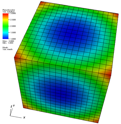
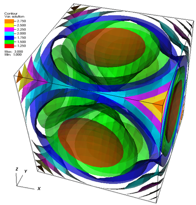
In three spatial dimensions, visualization is a bit more difficult. The left picture shows the solution and the mesh it was computed on on the surface of the domain. This is nice, but it has the drawback that it completely hides what is happening on the inside. The picture on the right is an attempt at visualizing the interior as well, by showing surfaces where the solution has constant values (as indicated by the legend at the top left). Isosurface pictures look best if one makes the individual surfaces slightly transparent so that it is possible to see through them and see what's behind.
| 
|
Essentially the possibilities for playing around with the program are the same as for the previous one, except that they will now also apply to the 3d case. For inspiration read up on possible extensions in the documentation of step 3.
 1.8.11

