Reference documentation for deal.II version 9.1.0-pre
The step-50 tutorial program

This tutorial depends on step-16, step-40.

Table of contents
  1. Introduction
  2. The commented program
  1. Results
  2. The plain program

This program has evolved from a version originally written by Guido Kanschat in 2003. It has undergone significant revisions by Bärbel Janssen, Guido Kanschat and Wolfgang Bangerth in 2009 and 2010 to demonstrate multigrid algorithms on adaptively refined meshes.

Introduction

This example shows the basic usage of the multilevel functions in deal.II. It solves the same problem as used in step-6, but demonstrating the things one has to provide when using multigrid as a preconditioner. In particular, this requires that we define a hierarchy of levels, provide transfer operators from one level to the next and back, and provide representations of the Laplace operator on each level.

In order to allow sufficient flexibility in conjunction with systems of differential equations and block preconditioners, quite a few different objects have to be created before starting the multilevel method, although most of what needs to be done is provided by deal.II itself. These are

Most of these objects will only be needed inside the function that actually solves the linear system. There, these objects are combined in an object of type Multigrid, containing the implementation of the V-cycle, which is in turn used by the preconditioner PreconditionMG, ready for plug-in into a linear solver of the LAC library.

The multilevel method in deal.II follows in many respects the outlines of the various publications by James Bramble, Joseph Pasciak and Jinchao Xu (i.e. the "BPX" framework). In order to understand many of the options, a rough familiarity with their work is quite helpful.

However, in comparison to this framework, the implementation in deal.II has to take into account the fact that we want to solve linear systems on adaptively refined meshes. This leads to the complication that it isn't quite as clear any more what exactly a "level" in a multilevel hierarchy of a mesh is. The following image shows what we consider to be a "level":

hanging_nodes.png

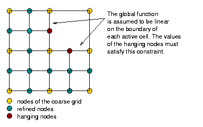
In other words, the fine level in this mesh consists only of the degrees of freedom that are defined on the refined cells, but does not extend to that part of the domain that is not refined. While this guarantees that the overall effort grows as \({\cal O}(N)\) as necessary for optimal multigrid complexity, it leads to problems when defining where to smooth and what boundary conditions to pose for the operators defined on individual levels if the level boundary is not an external boundary. These questions are discussed in detail in the Multigrid paper by Janssen and Kanschat that describes the implementation in deal.II.

The testcase

The problem we solve here is exactly the same as in step-6, the only difference being the solver we use here. You may want to look there for a definition of what we solve, right hand side and boundary conditions. Obviously, the program would also work if we changed the geometry and other pieces of data that defines this particular problem.

The things that are new are all those parts that concern the multigrid. In particular, this includes the following members of the main class:

Note
: This a work in progress example of parallel geometric multigrid. Some parts are still in heavy development.

This program is a parallel version of step-16 with a slightly different problem setup.

Include files

Again, the first few include files are already known, so we won't comment on them:

#include <deal.II/base/quadrature_lib.h>
#include <deal.II/base/function.h>
#include <deal.II/base/logstream.h>
#include <deal.II/base/utilities.h>
#include <deal.II/base/conditional_ostream.h>
#include <deal.II/lac/affine_constraints.h>
#include <deal.II/lac/vector.h>
#include <deal.II/lac/full_matrix.h>
#include <deal.II/lac/sparse_matrix.h>
#include <deal.II/lac/solver_cg.h>
#include <deal.II/lac/solver_gmres.h>
#include <deal.II/lac/precondition.h>
#include <deal.II/grid/tria.h>
#include <deal.II/grid/tria_accessor.h>
#include <deal.II/grid/tria_iterator.h>
#include <deal.II/grid/grid_generator.h>
#include <deal.II/grid/grid_out.h>
#include <deal.II/grid/grid_refinement.h>
#include <deal.II/dofs/dof_accessor.h>
#include <deal.II/dofs/dof_tools.h>
#include <deal.II/fe/fe_q.h>
#include <deal.II/fe/fe_values.h>
#include <deal.II/numerics/vector_tools.h>
#include <deal.II/numerics/data_out.h>
#include <deal.II/numerics/error_estimator.h>
#include <deal.II/base/index_set.h>
#include <deal.II/distributed/tria.h>
#include <deal.II/distributed/grid_refinement.h>
#include <deal.II/multigrid/mg_constrained_dofs.h>
#include <deal.II/multigrid/multigrid.h>
#include <deal.II/multigrid/mg_transfer.h>
#include <deal.II/multigrid/mg_tools.h>
#include <deal.II/multigrid/mg_coarse.h>
#include <deal.II/multigrid/mg_smoother.h>
#include <deal.II/multigrid/mg_matrix.h>
#include <deal.II/lac/generic_linear_algebra.h>

#define USE_PETSC_LA PETSc is not quite supported yet

namespace LA
{
#ifdef USE_PETSC_LA
using namespace ::LinearAlgebraPETSc;
#else
using namespace ::LinearAlgebraTrilinos;
#endif
} // namespace LA

This is C++:

#include <iostream>
#include <fstream>

The last step is as in all previous programs:

namespace Step50
{
using namespace dealii;

The LaplaceProblem class template

This main class is very similar to step-16, except that we are storing a parallel Triangulation and parallel versions of matrices and vectors.

template <int dim>
class LaplaceProblem
{
public:
LaplaceProblem(const unsigned int deg);
void run();
private:
void setup_system();
void assemble_system();
void assemble_multigrid();
void solve();
void refine_grid();
void output_results(const unsigned int cycle) const;
DoFHandler<dim> mg_dof_handler;
using matrix_t = LA::MPI::SparseMatrix;
using vector_t = LA::MPI::Vector;
matrix_t system_matrix;
IndexSet locally_relevant_set;
vector_t solution;
vector_t system_rhs;
const unsigned int degree;

Finally we are storing the various parallel multigrid matrices. Our problem is self-adjoint, so the interface matrices are the transpose of each other, so we only need to compute/store them once.

MGLevelObject<matrix_t> mg_interface_matrices;
MGConstrainedDoFs mg_constrained_dofs;
};

Nonconstant coefficients

The implementation of nonconstant coefficients is copied verbatim from step-5 and step-6:

template <int dim>
class Coefficient : public Function<dim>
{
public:
Coefficient()
: Function<dim>()
{}
virtual double value(const Point<dim> & p,
const unsigned int component = 0) const override;
virtual void value_list(const std::vector<Point<dim>> &points,
std::vector<double> & values,
const unsigned int component = 0) const override;
};
template <int dim>
double Coefficient<dim>::value(const Point<dim> &p, const unsigned int) const
{
if (p.square() < 0.5 * 0.5)
return 5;
else
return 1;
}
template <int dim>
void Coefficient<dim>::value_list(const std::vector<Point<dim>> &points,
std::vector<double> & values,
const unsigned int component) const
{
(void)component;
const unsigned int n_points = points.size();
Assert(values.size() == n_points,
ExcDimensionMismatch(values.size(), n_points));
Assert(component == 0, ExcIndexRange(component, 0, 1));
for (unsigned int i = 0; i < n_points; ++i)
values[i] = Coefficient<dim>::value(points[i]);
}

The LaplaceProblem class implementation

LaplaceProblem::LaplaceProblem

The constructor is left mostly unchanged. We take the polynomial degree of the finite elements to be used as a constructor argument and store it in a member variable.

By convention, all adaptively refined triangulations in deal.II never change by more than one level across a face between cells. For our multigrid algorithms, however, we need a slightly stricter guarantee, namely that the mesh also does not change by more than refinement level across vertices that might connect two cells. In other words, we must prevent the following situation:

limit_level_difference_at_vertices.png

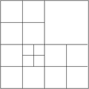
This is achieved by passing the Triangulation::limit_level_difference_at_vertices flag to the constructor of the triangulation class.

template <int dim>
LaplaceProblem<dim>::LaplaceProblem(const unsigned int degree)
: pcout(std::cout, (Utilities::MPI::this_mpi_process(MPI_COMM_WORLD) == 0))
, triangulation(MPI_COMM_WORLD,
Triangulation<dim>::limit_level_difference_at_vertices,
parallel::distributed::Triangulation<
dim>::construct_multigrid_hierarchy)
, fe(degree)
, mg_dof_handler(triangulation)
, degree(degree)
{}

LaplaceProblem::setup_system

The following function extends what the corresponding one in step-6 did. The top part, apart from the additional output, does the same:

template <int dim>
void LaplaceProblem<dim>::setup_system()
{
mg_dof_handler.distribute_dofs(fe);
mg_dof_handler.distribute_mg_dofs();
locally_relevant_set);
solution.reinit(mg_dof_handler.locally_owned_dofs(), MPI_COMM_WORLD);
system_rhs.reinit(mg_dof_handler.locally_owned_dofs(), MPI_COMM_WORLD);

But it starts to be a wee bit different here, although this still doesn't have anything to do with multigrid methods. step-6 took care of boundary values and hanging nodes in a separate step after assembling the global matrix from local contributions. This works, but the same can be done in a slightly simpler way if we already take care of these constraints at the time of copying local contributions into the global matrix. To this end, we here do not just compute the constraints do to hanging nodes, but also due to zero boundary conditions. We will use this set of constraints later on to help us copy local contributions correctly into the global linear system right away, without the need for a later clean-up stage:

constraints.reinit(locally_relevant_set);
DoFTools::make_hanging_node_constraints(mg_dof_handler, constraints);
std::set<types::boundary_id> dirichlet_boundary_ids;
std::map<types::boundary_id, const Function<dim> *> dirichlet_boundary;
Functions::ConstantFunction<dim> homogeneous_dirichlet_bc(1.0);
dirichlet_boundary_ids.insert(0);
dirichlet_boundary[0] = &homogeneous_dirichlet_bc;
dirichlet_boundary,
constraints);
constraints.close();
DynamicSparsityPattern dsp(mg_dof_handler.n_dofs(),
mg_dof_handler.n_dofs());
DoFTools::make_sparsity_pattern(mg_dof_handler, dsp, constraints);
system_matrix.reinit(mg_dof_handler.locally_owned_dofs(),
dsp,
MPI_COMM_WORLD,
true);

The multigrid constraints have to be initialized. They need to know about the boundary values as well, so we pass the dirichlet_boundary here as well.

mg_constrained_dofs.clear();
mg_constrained_dofs.initialize(mg_dof_handler);
mg_constrained_dofs.make_zero_boundary_constraints(mg_dof_handler,
dirichlet_boundary_ids);

Now for the things that concern the multigrid data structures. First, we resize the multilevel objects to hold matrices and sparsity patterns for every level. The coarse level is zero (this is mandatory right now but may change in a future revision). Note that these functions take a complete, inclusive range here (not a starting index and size), so the finest level is n_levels-1. We first have to resize the container holding the SparseMatrix classes, since they have to release their SparsityPattern before the can be destroyed upon resizing.

const unsigned int n_levels = triangulation.n_global_levels();
mg_interface_matrices.resize(0, n_levels - 1);
mg_interface_matrices.clear_elements();
mg_matrices.resize(0, n_levels - 1);
mg_matrices.clear_elements();

Now, we have to provide a matrix on each level. To this end, we first use the MGTools::make_sparsity_pattern function to first generate a preliminary compressed sparsity pattern on each level (see the Sparsity patterns module for more information on this topic) and then copy it over to the one we really want. The next step is to initialize both kinds of level matrices with these sparsity patterns.

It may be worth pointing out that the interface matrices only have entries for degrees of freedom that sit at or next to the interface between coarser and finer levels of the mesh. They are therefore even sparser than the matrices on the individual levels of our multigrid hierarchy. If we were more concerned about memory usage (and possibly the speed with which we can multiply with these matrices), we should use separate and different sparsity patterns for these two kinds of matrices.

for (unsigned int level = 0; level < n_levels; ++level)
{
DynamicSparsityPattern dsp(mg_dof_handler.n_dofs(level),
mg_dof_handler.n_dofs(level));
MGTools::make_sparsity_pattern(mg_dof_handler, dsp, level);
mg_matrices[level].reinit(mg_dof_handler.locally_owned_mg_dofs(level),
mg_dof_handler.locally_owned_mg_dofs(level),
dsp,
MPI_COMM_WORLD,
true);
mg_interface_matrices[level].reinit(
mg_dof_handler.locally_owned_mg_dofs(level),
dsp,
MPI_COMM_WORLD,
true);
}
}

LaplaceProblem::assemble_system

The following function assembles the linear system on the finest level of the mesh. It is almost exactly the same as in step-6, with the exception that we don't eliminate hanging nodes and boundary values after assembling, but while copying local contributions into the global matrix. This is not only simpler but also more efficient for large problems.

This latter trick is something that only found its way into deal.II over time and wasn't used in the initial version of this tutorial program. There is, however, a discussion of this function in the introduction of step-27.

template <int dim>
void LaplaceProblem<dim>::assemble_system()
{
const QGauss<dim> quadrature_formula(degree + 1);
FEValues<dim> fe_values(fe,
quadrature_formula,
const unsigned int dofs_per_cell = fe.dofs_per_cell;
const unsigned int n_q_points = quadrature_formula.size();
FullMatrix<double> cell_matrix(dofs_per_cell, dofs_per_cell);
Vector<double> cell_rhs(dofs_per_cell);
std::vector<types::global_dof_index> local_dof_indices(dofs_per_cell);
const Coefficient<dim> coefficient;
std::vector<double> coefficient_values(n_q_points);
for (const auto &cell : mg_dof_handler.active_cell_iterators())
if (cell->is_locally_owned())
{
cell_matrix = 0;
cell_rhs = 0;
fe_values.reinit(cell);
coefficient.value_list(fe_values.get_quadrature_points(),
coefficient_values);
for (unsigned int q_point = 0; q_point < n_q_points; ++q_point)
for (unsigned int i = 0; i < dofs_per_cell; ++i)
{
for (unsigned int j = 0; j < dofs_per_cell; ++j)
cell_matrix(i, j) +=
(coefficient_values[q_point] *
fe_values.shape_grad(i, q_point) *
fe_values.shape_grad(j, q_point) * fe_values.JxW(q_point));
cell_rhs(i) += (fe_values.shape_value(i, q_point) * 10.0 *
fe_values.JxW(q_point));
}
cell->get_dof_indices(local_dof_indices);
constraints.distribute_local_to_global(cell_matrix,
cell_rhs,
local_dof_indices,
system_matrix,
system_rhs);
}
system_matrix.compress(VectorOperation::add);
}

LaplaceProblem::assemble_multigrid

The next function is the one that builds the linear operators (matrices) that define the multigrid method on each level of the mesh. The integration core is the same as above, but the loop below will go over all existing cells instead of just the active ones, and the results must be entered into the correct matrix. Note also that since we only do multilevel preconditioning, no right-hand side needs to be assembled here.

Before we go there, however, we have to take care of a significant amount of book keeping:

template <int dim>
void LaplaceProblem<dim>::assemble_multigrid()
{
QGauss<dim> quadrature_formula(1 + degree);
FEValues<dim> fe_values(fe,
quadrature_formula,
const unsigned int dofs_per_cell = fe.dofs_per_cell;
const unsigned int n_q_points = quadrature_formula.size();
FullMatrix<double> cell_matrix(dofs_per_cell, dofs_per_cell);
std::vector<types::global_dof_index> local_dof_indices(dofs_per_cell);
const Coefficient<dim> coefficient;
std::vector<double> coefficient_values(n_q_points);

Next a few things that are specific to building the multigrid data structures (since we only need them in the current function, rather than also elsewhere, we build them here instead of the setup_system function). Some of the following may be a bit obscure if you're not familiar with the algorithm actually implemented in deal.II to support multilevel algorithms on adaptive meshes; if some of the things below seem strange, take a look at the mg_paper.

Our first job is to identify those degrees of freedom on each level that are located on interfaces between adaptively refined levels, and those that lie on the interface but also on the exterior boundary of the domain. The MGConstrainedDoFs already computed the information for us when we called initialize in

setup_system(). of type IndexSet on each level (get_refinement_edge_indices(),

The indices just identified will later be used to decide where the assembled value has to be added into on each level. On the other hand, we also have to impose zero boundary conditions on the external boundary of each level. But this the MGConstrainedDoFs knows it. So we simply ask for them by calling get_boundary_indices (). The third step is to construct constraints on all those degrees of freedom: their value should be zero after each application of the level operators. To this end, we construct AffineConstraints objects for each level, and add to each of these constraints for each degree of freedom. Due to the way the AffineConstraints class stores its data, the function to add a constraint on a single degree of freedom and force it to be zero is called AffineConstraints::add_line(); doing so for several degrees of freedom at once can be done using AffineConstraints::add_lines():

std::vector<AffineConstraints<double>> boundary_constraints(
triangulation.n_global_levels());
AffineConstraints<double> empty_constraints;
for (unsigned int level = 0; level < triangulation.n_global_levels();
++level)
{
IndexSet dofset;
level,
dofset);
boundary_constraints[level].reinit(dofset);
boundary_constraints[level].add_lines(
mg_constrained_dofs.get_refinement_edge_indices(level));
boundary_constraints[level].add_lines(
mg_constrained_dofs.get_boundary_indices(level));
boundary_constraints[level].close();
}

Now that we're done with most of our preliminaries, let's start the integration loop. It looks mostly like the loop in assemble_system, with two exceptions: (i) we don't need a right hand side, and more significantly (ii) we don't just loop over all active cells, but in fact all cells, active or not. Consequently, the correct iterator to use is DoFHandler::cell_iterator rather than DoFHandler::active_cell_iterator. Let's go about it:

for (const auto &cell : mg_dof_handler.active_cell_iterators())
if (cell->level_subdomain_id() == triangulation.locally_owned_subdomain())
{
cell_matrix = 0;
fe_values.reinit(cell);
coefficient.value_list(fe_values.get_quadrature_points(),
coefficient_values);
for (unsigned int q_point = 0; q_point < n_q_points; ++q_point)
for (unsigned int i = 0; i < dofs_per_cell; ++i)
for (unsigned int j = 0; j < dofs_per_cell; ++j)
cell_matrix(i, j) +=
(coefficient_values[q_point] *
fe_values.shape_grad(i, q_point) *
fe_values.shape_grad(j, q_point) * fe_values.JxW(q_point));

The rest of the assembly is again slightly different. This starts with a gotcha that is easily forgotten: The indices of global degrees of freedom we want here are the ones for current level, not for the global matrix. We therefore need the function MGDoFAccessorLLget_mg_dof_indices, not MGDoFAccessor::get_dof_indices as used in the assembly of the global system:

cell->get_mg_dof_indices(local_dof_indices);

Next, we need to copy local contributions into the level objects. We can do this in the same way as in the global assembly, using a constraint object that takes care of constrained degrees (which here are only boundary nodes, as the individual levels have no hanging node constraints). Note that the boundary_constraints object makes sure that the level matrices contains no contributions from degrees of freedom at the interface between cells of different refinement level.

boundary_constraints[cell->level()].distribute_local_to_global(
cell_matrix, local_dof_indices, mg_matrices[cell->level()]);

The next step is again slightly more obscure (but explained in the mg_paper): We need the remainder of the operator that we just copied into the mg_matrices object, namely the part on the interface between cells at the current level and cells one level coarser. This matrix exists in two directions: for interior DoFs (index \(i\)) of the current level to those sitting on the interface (index \(j\)), and the other way around. Of course, since we have a symmetric operator, one of these matrices is the transpose of the other.

The way we assemble these matrices is as follows: since the are formed from parts of the local contributions, we first delete all those parts of the local contributions that we are not interested in, namely all those elements of the local matrix for which not \(i\) is an interface DoF and \(j\) is not. The result is one of the two matrices that we are interested in, and we then copy it into the mg_interface_matrices object. The boundary_interface_constraints object at the same time makes sure that we delete contributions from all degrees of freedom that are not only on the interface but also on the external boundary of the domain.

The last part to remember is how to get the other matrix. Since it is only the transpose, we will later (in the solve() function) be able to just pass the transpose matrix where necessary.

const IndexSet &interface_dofs_on_level =
mg_constrained_dofs.get_refinement_edge_indices(cell->level());
const unsigned int lvl = cell->level();
for (unsigned int i = 0; i < dofs_per_cell; ++i)
for (unsigned int j = 0; j < dofs_per_cell; ++j)
if (interface_dofs_on_level.is_element(
local_dof_indices[i]) // at_refinement_edge(i)
&& !interface_dofs_on_level.is_element(
local_dof_indices[j]) // !at_refinement_edge(j)
&&
((!mg_constrained_dofs.is_boundary_index(
lvl, local_dof_indices[i]) &&
!mg_constrained_dofs.is_boundary_index(
lvl,
local_dof_indices[j])) // ( !boundary(i) && !boundary(j) )
|| (mg_constrained_dofs.is_boundary_index(
lvl, local_dof_indices[i]) &&
local_dof_indices[i] ==
local_dof_indices[j]) // ( boundary(i) && boundary(j)

&& i==j )

))
{

do nothing, so add entries to interface matrix

}
else
{
cell_matrix(i, j) = 0;
}
empty_constraints.distribute_local_to_global(
cell_matrix,
local_dof_indices,
mg_interface_matrices[cell->level()]);
}
for (unsigned int i = 0; i < triangulation.n_global_levels(); ++i)
{
mg_matrices[i].compress(VectorOperation::add);
mg_interface_matrices[i].compress(VectorOperation::add);
}
}

LaplaceProblem::solve

This is the other function that is significantly different in support of the multigrid solver (or, in fact, the preconditioner for which we use the multigrid method).

Let us start out by setting up two of the components of multilevel methods: transfer operators between levels, and a solver on the coarsest level. In finite element methods, the transfer operators are derived from the finite element function spaces involved and can often be computed in a generic way independent of the problem under consideration. In that case, we can use the MGTransferPrebuilt class that, given the constraints on the global level and an DoFHandler object computes the matrices corresponding to these transfer operators.

The second part of the following lines deals with the coarse grid solver. Since our coarse grid is very coarse indeed, we decide for a direct solver (a Householder decomposition of the coarsest level matrix), even if its implementation is not particularly sophisticated. If our coarse mesh had many more cells than the five we have here, something better suited would obviously be necessary here.

template <int dim>
void LaplaceProblem<dim>::solve()
{

Create the object that deals with the transfer between different refinement levels.

MGTransferPrebuilt<vector_t> mg_transfer(mg_constrained_dofs);

Now the prolongation matrix has to be built.

mg_transfer.build_matrices(mg_dof_handler);
matrix_t &coarse_matrix = mg_matrices[0];
SolverControl coarse_solver_control(1000, 1e-10, false, false);
SolverCG<vector_t> coarse_solver(coarse_solver_control);
matrix_t,
coarse_grid_solver(coarse_solver, coarse_matrix, id);

The next component of a multilevel solver or preconditioner is that we need a smoother on each level. A common choice for this is to use the application of a relaxation method (such as the SOR, Jacobi or Richardson method). The MGSmootherPrecondition class provides support for this kind of smoother. Here, we opt for the application of a single SOR iteration. To this end, we define an appropriate alias and then setup a smoother object.

The last step is to initialize the smoother object with our level matrices and to set some smoothing parameters. The initialize() function can optionally take additional arguments that will be passed to the smoother object on each level. In the current case for the SOR smoother, this could, for example, include a relaxation parameter. However, we here leave these at their default values. The call to set_steps() indicates that we will use two pre- and two post-smoothing steps on each level; to use a variable number of smoother steps on different levels, more options can be set in the constructor call to the mg_smoother object.

The last step results from the fact that we use the SOR method as a smoother - which is not symmetric - but we use the conjugate gradient iteration (which requires a symmetric preconditioner) below, we need to let the multilevel preconditioner make sure that we get a symmetric operator even for nonsymmetric smoothers:

using Smoother = LA::MPI::PreconditionJacobi;
mg_smoother.initialize(mg_matrices, Smoother::AdditionalData(0.5));
mg_smoother.set_steps(2);

mg_smoother.set_symmetric(false);

The next preparatory step is that we must wrap our level and interface matrices in an object having the required multiplication functions. We will create two objects for the interface objects going from coarse to fine and the other way around; the multigrid algorithm will later use the transpose operator for the latter operation, allowing us to initialize both up and down versions of the operator with the matrices we already built:

mg::Matrix<vector_t> mg_matrix(mg_matrices);
mg::Matrix<vector_t> mg_interface_up(mg_interface_matrices);
mg::Matrix<vector_t> mg_interface_down(mg_interface_matrices);

Now, we are ready to set up the V-cycle operator and the multilevel preconditioner.

mg_matrix, coarse_grid_solver, mg_transfer, mg_smoother, mg_smoother);

mg.set_debug(6);

mg.set_edge_matrices(mg_interface_down, mg_interface_up);
mg_dof_handler, mg, mg_transfer);

With all this together, we can finally get about solving the linear system in the usual way:

SolverControl solver_control(500, 1e-8 * system_rhs.l2_norm(), false);
SolverCG<vector_t> solver(solver_control);
if (false)
{
/ *

code to optionally compare to Trilinos ML

TrilinosWrappers::PreconditionAMG prec;

Amg_data.constant_modes = constant_modes;

Amg_data.elliptic = true;
Amg_data.higher_order_elements = true;
Amg_data.smoother_sweeps = 2;
Amg_data.aggregation_threshold = 0.02;

Amg_data.symmetric = true;

prec.initialize (system_matrix,
Amg_data);
solver.solve (system_matrix, solution, system_rhs, prec);
* /
}
else
{
solver.solve(system_matrix, solution, system_rhs, preconditioner);
}
pcout << " CG converged in " << solver_control.last_step()
<< " iterations." << std::endl;
constraints.distribute(solution);
}

Postprocessing

The following two functions postprocess a solution once it is computed. In particular, the first one refines the mesh at the beginning of each cycle while the second one outputs results at the end of each such cycle. The refine_grid() method is almost unchanged from step-6: the only substantial difference is that this method uses a distributed grid refinement function instead of a serial one. The output_results() method is quite different since each processor writes only part of the overall graphical output.

template <int dim>
void LaplaceProblem<dim>::refine_grid()
{
Vector<float> estimated_error_per_cell(triangulation.n_active_cells());
LA::MPI::Vector temp_solution;
temp_solution.reinit(locally_relevant_set, MPI_COMM_WORLD);
temp_solution = solution;
mg_dof_handler,
QGauss<dim - 1>(degree + 1),
std::map<types::boundary_id, const Function<dim> *>(),
temp_solution,
estimated_error_per_cell);
triangulation, estimated_error_per_cell, 0.3, 0.0);
}
template <int dim>
void LaplaceProblem<dim>::output_results(const unsigned int cycle) const
{
DataOut<dim> data_out;
LA::MPI::Vector temp_solution;
temp_solution.reinit(locally_relevant_set, MPI_COMM_WORLD);
temp_solution = solution;
LA::MPI::Vector temp = solution;
system_matrix.residual(temp, solution, system_rhs);
LA::MPI::Vector res_ghosted = temp_solution;
res_ghosted = temp;
data_out.attach_dof_handler(mg_dof_handler);
data_out.add_data_vector(temp_solution, "solution");
data_out.add_data_vector(res_ghosted, "res");
Vector<float> subdomain(triangulation.n_active_cells());
for (unsigned int i = 0; i < subdomain.size(); ++i)
subdomain(i) = triangulation.locally_owned_subdomain();
data_out.add_data_vector(subdomain, "subdomain");
data_out.build_patches(0);
const std::string filename =
("solution-" + Utilities::int_to_string(cycle, 5) + "." +
".vtu");
std::ofstream output(filename);
data_out.write_vtu(output);
if (Utilities::MPI::this_mpi_process(MPI_COMM_WORLD) == 0)
{
std::vector<std::string> filenames;
for (unsigned int i = 0;
i < Utilities::MPI::n_mpi_processes(MPI_COMM_WORLD);
++i)
filenames.push_back(std::string("solution-") +
Utilities::int_to_string(cycle, 5) + "." +
Utilities::int_to_string(i, 4) + ".vtu");
const std::string pvtu_master_filename =
("solution-" + Utilities::int_to_string(cycle, 5) + ".pvtu");
std::ofstream pvtu_master(pvtu_master_filename);
data_out.write_pvtu_record(pvtu_master, filenames);
const std::string visit_master_filename =
("solution-" + Utilities::int_to_string(cycle, 5) + ".visit");
std::ofstream visit_master(visit_master_filename);
DataOutBase::write_visit_record(visit_master, filenames);
std::cout << " wrote " << pvtu_master_filename << std::endl;
}
}

LaplaceProblem::run

Like several of the functions above, this is almost exactly a copy of the corresponding function in step-6. The only difference is the call to assemble_multigrid that takes care of forming the matrices on every level that we need in the multigrid method.

template <int dim>
void LaplaceProblem<dim>::run()
{
for (unsigned int cycle = 0; cycle < 15; ++cycle)
{
pcout << "Cycle " << cycle << ':' << std::endl;
if (cycle == 0)
{
GridGenerator::hyper_cube(triangulation);
triangulation.refine_global(4);
}
else
refine_grid();
pcout << " Number of active cells: "
<< triangulation.n_global_active_cells() << std::endl;
setup_system();
pcout << " Number of degrees of freedom: " << mg_dof_handler.n_dofs()
<< " (by level: ";
for (unsigned int level = 0; level < triangulation.n_global_levels();
++level)
pcout << mg_dof_handler.n_dofs(level)
<< (level == triangulation.n_global_levels() - 1 ? ")" : ", ");
pcout << std::endl;
assemble_system();
assemble_multigrid();
solve();
output_results(cycle);
}
}
} // namespace Step50

The main() function

This is again the same function as in step-6:

int main(int argc, char *argv[])
{
try
{
using namespace dealii;
using namespace Step50;
Utilities::MPI::MPI_InitFinalize mpi_initialization(argc, argv, 1);
LaplaceProblem<2> laplace_problem(1 / *degree* /);
laplace_problem.run();
}
catch (std::exception &exc)
{
std::cerr << std::endl
<< std::endl
<< "----------------------------------------------------"
<< std::endl;
std::cerr << "Exception on processing: " << std::endl
<< exc.what() << std::endl
<< "Aborting!" << std::endl
<< "----------------------------------------------------"
<< std::endl;
}
catch (...)
{
std::cerr << std::endl
<< std::endl
<< "----------------------------------------------------"
<< std::endl;
std::cerr << "Unknown exception!" << std::endl
<< "Aborting!" << std::endl
<< "----------------------------------------------------"
<< std::endl;
throw;
}
return 0;
}

Results

The output that this program generates is, of course, the same as that of step-6, so you may see there for more results. On the other hand, since no tutorial program is a good one unless it has at least one colorful picture, here is, again, the solution:

When run, the output of this program is

Cycle 0:
   Number of active cells:       20
   Number of degrees of freedom: 25 (by level: 8, 25)
   7 CG iterations needed to obtain convergence.
Cycle 1:
   Number of active cells:       44
   Number of degrees of freedom: 57 (by level: 8, 25, 48)
   8 CG iterations needed to obtain convergence.
Cycle 2:
   Number of active cells:       92
   Number of degrees of freedom: 117 (by level: 8, 25, 80, 60)
   9 CG iterations needed to obtain convergence.
Cycle 3:
   Number of active cells:       188
   Number of degrees of freedom: 221 (by level: 8, 25, 80, 200)
   12 CG iterations needed to obtain convergence.
Cycle 4:
   Number of active cells:       416
   Number of degrees of freedom: 485 (by level: 8, 25, 89, 288, 280)
   13 CG iterations needed to obtain convergence.
Cycle 5:
   Number of active cells:       800
   Number of degrees of freedom: 925 (by level: 8, 25, 89, 288, 784, 132)
   14 CG iterations needed to obtain convergence.
Cycle 6:
   Number of active cells:       1628
   Number of degrees of freedom: 1865 (by level: 8, 25, 89, 304, 1000, 1164, 72)
   14 CG iterations needed to obtain convergence.
Cycle 7:
   Number of active cells:       3194
   Number of degrees of freedom: 3603 (by level: 8, 25, 89, 328, 1032, 2200, 1392)
   16 CG iterations needed to obtain convergence.

That's not perfect — we would have hoped for a constant number of iterations rather than one that increases as we get more and more degrees of freedom — but it is also not far away. The reason for this is easy enough to understand, however: since we have a strongly varying coefficient, the operators that we assembly by quadrature on the lower levels become worse and worse approximations of the operator on the finest level. Consequently, even if we had perfect solvers on the coarser levels, they would not be good preconditioners on the finest level. This theory is easily tested by comparing results when we use a constant coefficient: in that case, the number of iterations remains constant at 9 after the first three or four refinement steps.

We can also compare what this program produces with how step-5 performed. To solve the same problem as in step-5, the only two changes that are necessary are (i) to replace the body of the function LaplaceProblem::refine_grid by a call to triangulation.refine_global(1), and (ii) to use the same SolverControl object and tolerance as in step-5 — the rest of the program remains unchanged. In that case, here is how the solvers used in step-5 and the multigrid solver used in the current program compare:

cellsstep-5step-16
20 13 6
80 17 7
320 29 9
1280 51 10
5120 94 11
2048018013

This isn't only fewer iterations than in step-5 (each of which is, however, much more expensive) but more importantly, the number of iterations also grows much more slowly under mesh refinement (again, it would be almost constant if the coefficient was constant rather than strongly varying as chosen here). This justifies the common observation that, whenever possible, multigrid methods should be used for second order problems.

Possible extensions

A close inspection of this program's performance shows that it is mostly dominated by matrix-vector operations. step-37 shows one way how this can be avoided by working with matrix-free methods.

Another avenue would be to use algebraic multigrid methods. The geometric multigrid method used here can at times be a bit awkward to implement because it needs all those additional data structures, and it becomes even more difficult if the program is to run in parallel on machines coupled through MPI, for example. In that case, it would be simpler if one could use a black-box preconditioner that uses some sort of multigrid hierarchy for good performance but can figure out level matrices and similar things out by itself. Algebraic multigrid methods do exactly this, and we will use them in step-31 for the solution of a Stokes problem.

The plain program

/* ---------------------------------------------------------------------
*
* Copyright (C) 2003 - 2018 by the deal.II authors
*
* This file is part of the deal.II library.
*
* The deal.II library is free software; you can use it, redistribute
* it, and/or modify it under the terms of the GNU Lesser General
* Public License as published by the Free Software Foundation; either
* version 2.1 of the License, or (at your option) any later version.
* The full text of the license can be found in the file LICENSE.md at
* the top level directory of deal.II.
*
* ---------------------------------------------------------------------
*
* Author: Guido Kanschat and Timo Heister
*/
#include <deal.II/base/quadrature_lib.h>
#include <deal.II/base/function.h>
#include <deal.II/base/logstream.h>
#include <deal.II/base/utilities.h>
#include <deal.II/base/conditional_ostream.h>
#include <deal.II/lac/affine_constraints.h>
#include <deal.II/lac/vector.h>
#include <deal.II/lac/full_matrix.h>
#include <deal.II/lac/sparse_matrix.h>
#include <deal.II/lac/solver_cg.h>
#include <deal.II/lac/solver_gmres.h>
#include <deal.II/lac/precondition.h>
#include <deal.II/grid/tria.h>
#include <deal.II/grid/tria_accessor.h>
#include <deal.II/grid/tria_iterator.h>
#include <deal.II/grid/grid_generator.h>
#include <deal.II/grid/grid_out.h>
#include <deal.II/grid/grid_refinement.h>
#include <deal.II/dofs/dof_accessor.h>
#include <deal.II/dofs/dof_tools.h>
#include <deal.II/fe/fe_q.h>
#include <deal.II/fe/fe_values.h>
#include <deal.II/numerics/vector_tools.h>
#include <deal.II/numerics/data_out.h>
#include <deal.II/numerics/error_estimator.h>
#include <deal.II/base/index_set.h>
#include <deal.II/distributed/tria.h>
#include <deal.II/distributed/grid_refinement.h>
#include <deal.II/multigrid/mg_constrained_dofs.h>
#include <deal.II/multigrid/multigrid.h>
#include <deal.II/multigrid/mg_transfer.h>
#include <deal.II/multigrid/mg_tools.h>
#include <deal.II/multigrid/mg_coarse.h>
#include <deal.II/multigrid/mg_smoother.h>
#include <deal.II/multigrid/mg_matrix.h>
#include <deal.II/lac/generic_linear_algebra.h>
namespace LA
{
#ifdef USE_PETSC_LA
using namespace ::LinearAlgebraPETSc;
#else
using namespace ::LinearAlgebraTrilinos;
#endif
} // namespace LA
#include <iostream>
#include <fstream>
namespace Step50
{
using namespace dealii;
template <int dim>
class LaplaceProblem
{
public:
LaplaceProblem(const unsigned int deg);
void run();
private:
void setup_system();
void assemble_system();
void assemble_multigrid();
void solve();
void refine_grid();
void output_results(const unsigned int cycle) const;
DoFHandler<dim> mg_dof_handler;
using matrix_t = LA::MPI::SparseMatrix;
using vector_t = LA::MPI::Vector;
matrix_t system_matrix;
IndexSet locally_relevant_set;
vector_t solution;
vector_t system_rhs;
const unsigned int degree;
MGLevelObject<matrix_t> mg_interface_matrices;
MGConstrainedDoFs mg_constrained_dofs;
};
template <int dim>
class Coefficient : public Function<dim>
{
public:
Coefficient()
: Function<dim>()
{}
virtual double value(const Point<dim> & p,
const unsigned int component = 0) const override;
virtual void value_list(const std::vector<Point<dim>> &points,
std::vector<double> & values,
const unsigned int component = 0) const override;
};
template <int dim>
double Coefficient<dim>::value(const Point<dim> &p, const unsigned int) const
{
if (p.square() < 0.5 * 0.5)
return 5;
else
return 1;
}
template <int dim>
void Coefficient<dim>::value_list(const std::vector<Point<dim>> &points,
std::vector<double> & values,
const unsigned int component) const
{
(void)component;
const unsigned int n_points = points.size();
Assert(values.size() == n_points,
ExcDimensionMismatch(values.size(), n_points));
Assert(component == 0, ExcIndexRange(component, 0, 1));
for (unsigned int i = 0; i < n_points; ++i)
values[i] = Coefficient<dim>::value(points[i]);
}
template <int dim>
LaplaceProblem<dim>::LaplaceProblem(const unsigned int degree)
: pcout(std::cout, (Utilities::MPI::this_mpi_process(MPI_COMM_WORLD) == 0))
, triangulation(MPI_COMM_WORLD,
Triangulation<dim>::limit_level_difference_at_vertices,
parallel::distributed::Triangulation<
dim>::construct_multigrid_hierarchy)
, fe(degree)
, mg_dof_handler(triangulation)
, degree(degree)
{}
template <int dim>
void LaplaceProblem<dim>::setup_system()
{
mg_dof_handler.distribute_dofs(fe);
mg_dof_handler.distribute_mg_dofs();
locally_relevant_set);
solution.reinit(mg_dof_handler.locally_owned_dofs(), MPI_COMM_WORLD);
system_rhs.reinit(mg_dof_handler.locally_owned_dofs(), MPI_COMM_WORLD);
constraints.reinit(locally_relevant_set);
DoFTools::make_hanging_node_constraints(mg_dof_handler, constraints);
std::set<types::boundary_id> dirichlet_boundary_ids;
std::map<types::boundary_id, const Function<dim> *> dirichlet_boundary;
Functions::ConstantFunction<dim> homogeneous_dirichlet_bc(1.0);
dirichlet_boundary_ids.insert(0);
dirichlet_boundary[0] = &homogeneous_dirichlet_bc;
dirichlet_boundary,
constraints);
constraints.close();
DynamicSparsityPattern dsp(mg_dof_handler.n_dofs(),
mg_dof_handler.n_dofs());
DoFTools::make_sparsity_pattern(mg_dof_handler, dsp, constraints);
system_matrix.reinit(mg_dof_handler.locally_owned_dofs(),
dsp,
MPI_COMM_WORLD,
true);
mg_constrained_dofs.clear();
mg_constrained_dofs.initialize(mg_dof_handler);
mg_constrained_dofs.make_zero_boundary_constraints(mg_dof_handler,
dirichlet_boundary_ids);
const unsigned int n_levels = triangulation.n_global_levels();
mg_interface_matrices.resize(0, n_levels - 1);
mg_interface_matrices.clear_elements();
mg_matrices.resize(0, n_levels - 1);
mg_matrices.clear_elements();
for (unsigned int level = 0; level < n_levels; ++level)
{
DynamicSparsityPattern dsp(mg_dof_handler.n_dofs(level),
mg_dof_handler.n_dofs(level));
MGTools::make_sparsity_pattern(mg_dof_handler, dsp, level);
mg_matrices[level].reinit(mg_dof_handler.locally_owned_mg_dofs(level),
mg_dof_handler.locally_owned_mg_dofs(level),
dsp,
MPI_COMM_WORLD,
true);
mg_interface_matrices[level].reinit(
mg_dof_handler.locally_owned_mg_dofs(level),
dsp,
MPI_COMM_WORLD,
true);
}
}
template <int dim>
void LaplaceProblem<dim>::assemble_system()
{
const QGauss<dim> quadrature_formula(degree + 1);
FEValues<dim> fe_values(fe,
quadrature_formula,
const unsigned int dofs_per_cell = fe.dofs_per_cell;
const unsigned int n_q_points = quadrature_formula.size();
FullMatrix<double> cell_matrix(dofs_per_cell, dofs_per_cell);
Vector<double> cell_rhs(dofs_per_cell);
std::vector<types::global_dof_index> local_dof_indices(dofs_per_cell);
const Coefficient<dim> coefficient;
std::vector<double> coefficient_values(n_q_points);
for (const auto &cell : mg_dof_handler.active_cell_iterators())
if (cell->is_locally_owned())
{
cell_matrix = 0;
cell_rhs = 0;
fe_values.reinit(cell);
coefficient.value_list(fe_values.get_quadrature_points(),
coefficient_values);
for (unsigned int q_point = 0; q_point < n_q_points; ++q_point)
for (unsigned int i = 0; i < dofs_per_cell; ++i)
{
for (unsigned int j = 0; j < dofs_per_cell; ++j)
cell_matrix(i, j) +=
(coefficient_values[q_point] *
fe_values.shape_grad(i, q_point) *
fe_values.shape_grad(j, q_point) * fe_values.JxW(q_point));
cell_rhs(i) += (fe_values.shape_value(i, q_point) * 10.0 *
fe_values.JxW(q_point));
}
cell->get_dof_indices(local_dof_indices);
constraints.distribute_local_to_global(cell_matrix,
cell_rhs,
local_dof_indices,
system_matrix,
system_rhs);
}
system_matrix.compress(VectorOperation::add);
}
template <int dim>
void LaplaceProblem<dim>::assemble_multigrid()
{
QGauss<dim> quadrature_formula(1 + degree);
FEValues<dim> fe_values(fe,
quadrature_formula,
const unsigned int dofs_per_cell = fe.dofs_per_cell;
const unsigned int n_q_points = quadrature_formula.size();
FullMatrix<double> cell_matrix(dofs_per_cell, dofs_per_cell);
std::vector<types::global_dof_index> local_dof_indices(dofs_per_cell);
const Coefficient<dim> coefficient;
std::vector<double> coefficient_values(n_q_points);
std::vector<AffineConstraints<double>> boundary_constraints(
triangulation.n_global_levels());
AffineConstraints<double> empty_constraints;
for (unsigned int level = 0; level < triangulation.n_global_levels();
++level)
{
IndexSet dofset;
level,
dofset);
boundary_constraints[level].reinit(dofset);
boundary_constraints[level].add_lines(
mg_constrained_dofs.get_refinement_edge_indices(level));
boundary_constraints[level].add_lines(
mg_constrained_dofs.get_boundary_indices(level));
boundary_constraints[level].close();
}
for (const auto &cell : mg_dof_handler.active_cell_iterators())
if (cell->level_subdomain_id() == triangulation.locally_owned_subdomain())
{
cell_matrix = 0;
fe_values.reinit(cell);
coefficient.value_list(fe_values.get_quadrature_points(),
coefficient_values);
for (unsigned int q_point = 0; q_point < n_q_points; ++q_point)
for (unsigned int i = 0; i < dofs_per_cell; ++i)
for (unsigned int j = 0; j < dofs_per_cell; ++j)
cell_matrix(i, j) +=
(coefficient_values[q_point] *
fe_values.shape_grad(i, q_point) *
fe_values.shape_grad(j, q_point) * fe_values.JxW(q_point));
cell->get_mg_dof_indices(local_dof_indices);
boundary_constraints[cell->level()].distribute_local_to_global(
cell_matrix, local_dof_indices, mg_matrices[cell->level()]);
const IndexSet &interface_dofs_on_level =
mg_constrained_dofs.get_refinement_edge_indices(cell->level());
const unsigned int lvl = cell->level();
for (unsigned int i = 0; i < dofs_per_cell; ++i)
for (unsigned int j = 0; j < dofs_per_cell; ++j)
if (interface_dofs_on_level.is_element(
local_dof_indices[i]) // at_refinement_edge(i)
&& !interface_dofs_on_level.is_element(
local_dof_indices[j]) // !at_refinement_edge(j)
&&
((!mg_constrained_dofs.is_boundary_index(
lvl, local_dof_indices[i]) &&
!mg_constrained_dofs.is_boundary_index(
lvl,
local_dof_indices[j])) // ( !boundary(i) && !boundary(j) )
|| (mg_constrained_dofs.is_boundary_index(
lvl, local_dof_indices[i]) &&
local_dof_indices[i] ==
local_dof_indices[j]) // ( boundary(i) && boundary(j)
))
{
}
else
{
cell_matrix(i, j) = 0;
}
empty_constraints.distribute_local_to_global(
cell_matrix,
local_dof_indices,
mg_interface_matrices[cell->level()]);
}
for (unsigned int i = 0; i < triangulation.n_global_levels(); ++i)
{
mg_matrices[i].compress(VectorOperation::add);
mg_interface_matrices[i].compress(VectorOperation::add);
}
}
template <int dim>
void LaplaceProblem<dim>::solve()
{
MGTransferPrebuilt<vector_t> mg_transfer(mg_constrained_dofs);
mg_transfer.build_matrices(mg_dof_handler);
matrix_t &coarse_matrix = mg_matrices[0];
SolverControl coarse_solver_control(1000, 1e-10, false, false);
SolverCG<vector_t> coarse_solver(coarse_solver_control);
SolverCG<vector_t>,
matrix_t,
coarse_grid_solver(coarse_solver, coarse_matrix, id);
using Smoother = LA::MPI::PreconditionJacobi;
mg_smoother.initialize(mg_matrices, Smoother::AdditionalData(0.5));
mg_smoother.set_steps(2);
mg::Matrix<vector_t> mg_matrix(mg_matrices);
mg::Matrix<vector_t> mg_interface_up(mg_interface_matrices);
mg::Matrix<vector_t> mg_interface_down(mg_interface_matrices);
mg_matrix, coarse_grid_solver, mg_transfer, mg_smoother, mg_smoother);
mg.set_edge_matrices(mg_interface_down, mg_interface_up);
mg_dof_handler, mg, mg_transfer);
SolverControl solver_control(500, 1e-8 * system_rhs.l2_norm(), false);
SolverCG<vector_t> solver(solver_control);
if (false)
{
/*
TrilinosWrappers::PreconditionAMG prec;
TrilinosWrappers::PreconditionAMG::AdditionalData Amg_data;
Amg_data.elliptic = true;
Amg_data.higher_order_elements = true;
Amg_data.smoother_sweeps = 2;
Amg_data.aggregation_threshold = 0.02;
prec.initialize (system_matrix,
Amg_data);
solver.solve (system_matrix, solution, system_rhs, prec);
*/
}
else
{
solver.solve(system_matrix, solution, system_rhs, preconditioner);
}
pcout << " CG converged in " << solver_control.last_step()
<< " iterations." << std::endl;
constraints.distribute(solution);
}
template <int dim>
void LaplaceProblem<dim>::refine_grid()
{
Vector<float> estimated_error_per_cell(triangulation.n_active_cells());
LA::MPI::Vector temp_solution;
temp_solution.reinit(locally_relevant_set, MPI_COMM_WORLD);
temp_solution = solution;
mg_dof_handler,
QGauss<dim - 1>(degree + 1),
std::map<types::boundary_id, const Function<dim> *>(),
temp_solution,
estimated_error_per_cell);
triangulation, estimated_error_per_cell, 0.3, 0.0);
}
template <int dim>
void LaplaceProblem<dim>::output_results(const unsigned int cycle) const
{
DataOut<dim> data_out;
LA::MPI::Vector temp_solution;
temp_solution.reinit(locally_relevant_set, MPI_COMM_WORLD);
temp_solution = solution;
LA::MPI::Vector temp = solution;
system_matrix.residual(temp, solution, system_rhs);
LA::MPI::Vector res_ghosted = temp_solution;
res_ghosted = temp;
data_out.attach_dof_handler(mg_dof_handler);
data_out.add_data_vector(temp_solution, "solution");
data_out.add_data_vector(res_ghosted, "res");
Vector<float> subdomain(triangulation.n_active_cells());
for (unsigned int i = 0; i < subdomain.size(); ++i)
subdomain(i) = triangulation.locally_owned_subdomain();
data_out.add_data_vector(subdomain, "subdomain");
data_out.build_patches(0);
const std::string filename =
("solution-" + Utilities::int_to_string(cycle, 5) + "." +
".vtu");
std::ofstream output(filename);
data_out.write_vtu(output);
if (Utilities::MPI::this_mpi_process(MPI_COMM_WORLD) == 0)
{
std::vector<std::string> filenames;
for (unsigned int i = 0;
i < Utilities::MPI::n_mpi_processes(MPI_COMM_WORLD);
++i)
filenames.push_back(std::string("solution-") +
Utilities::int_to_string(cycle, 5) + "." +
Utilities::int_to_string(i, 4) + ".vtu");
const std::string pvtu_master_filename =
("solution-" + Utilities::int_to_string(cycle, 5) + ".pvtu");
std::ofstream pvtu_master(pvtu_master_filename);
data_out.write_pvtu_record(pvtu_master, filenames);
const std::string visit_master_filename =
("solution-" + Utilities::int_to_string(cycle, 5) + ".visit");
std::ofstream visit_master(visit_master_filename);
DataOutBase::write_visit_record(visit_master, filenames);
std::cout << " wrote " << pvtu_master_filename << std::endl;
}
}
template <int dim>
void LaplaceProblem<dim>::run()
{
for (unsigned int cycle = 0; cycle < 15; ++cycle)
{
pcout << "Cycle " << cycle << ':' << std::endl;
if (cycle == 0)
{
GridGenerator::hyper_cube(triangulation);
triangulation.refine_global(4);
}
else
refine_grid();
pcout << " Number of active cells: "
<< triangulation.n_global_active_cells() << std::endl;
setup_system();
pcout << " Number of degrees of freedom: " << mg_dof_handler.n_dofs()
<< " (by level: ";
for (unsigned int level = 0; level < triangulation.n_global_levels();
++level)
pcout << mg_dof_handler.n_dofs(level)
<< (level == triangulation.n_global_levels() - 1 ? ")" : ", ");
pcout << std::endl;
assemble_system();
assemble_multigrid();
solve();
output_results(cycle);
}
}
} // namespace Step50
int main(int argc, char *argv[])
{
try
{
using namespace dealii;
using namespace Step50;
Utilities::MPI::MPI_InitFinalize mpi_initialization(argc, argv, 1);
LaplaceProblem<2> laplace_problem(1 /*degree*/);
laplace_problem.run();
}
catch (std::exception &exc)
{
std::cerr << std::endl
<< std::endl
<< "----------------------------------------------------"
<< std::endl;
std::cerr << "Exception on processing: " << std::endl
<< exc.what() << std::endl
<< "Aborting!" << std::endl
<< "----------------------------------------------------"
<< std::endl;
}
catch (...)
{
std::cerr << std::endl
<< std::endl
<< "----------------------------------------------------"
<< std::endl;
std::cerr << "Unknown exception!" << std::endl
<< "Aborting!" << std::endl
<< "----------------------------------------------------"
<< std::endl;
throw;
}
return 0;
}